Risk and Uncertainty
Review of Probability Theory
Probability theory is the study of uncertainty and chance. We often have to make decisions where the outcome depends on unpredictable factors outside our control. Probability theory is therefore an important tool for studying economics.
Random variables
Probability theory deals with random variables. A random variable is simply a number that can take on many different values, with different chances of each value.
For example, if you roll a dice, the number that you get can be modeled as a random variable. If you flip a coin, whether you get a heads or tails can also be modeled as a random variable.
In finance, a common thing to model as a random variable is the price of a stock.
There are many things in life that are appropriately modeled as random variables.
Outcomes and probabilities over outcomes
A random variable has a set of possible outcomes. Each of those outcomes has a probability of occurring. The probability of an outcome is simply the chance that the random variable turns out to that outcome.
Example: Dice Roll
Let \(X\) be a random variable denoting the outcome of a dice roll. The possible outcomes of \(X\) are: \(1, 2, 3, 4, 5, 6\), and the probability of each outcome is \(\frac{1}{6}\).
Example: Flipping a coin
Let \(X\) be a random variable denoting the outcome of a coin flip. The possible outcomes of \(X\) are: Heads, Tails. The probability of Heads is \(\frac{1}{2}\) and the probability of Tails is \(\frac{1}{2}\).
This example demonstrates that the possible outcomes of a random variable don’t necessarily have to be numbers.
Mathematical Insight
The probabilities over the outcomes of a random variable must add up to \(1\). This is because if you add up the chances of each possible outcome occurring, they have to add up to \(100\%\)!
Expected value
Let \(X\) be a numeric random variable with possible outcomes \(x_1, x_2, \ldots, x_N\). The probability of each of those outcomes is \(p_1, p_1, \ldots, p_N\).
The expected value of \(X\), which we write as \(E[X]\), is defined as:
\[\begin{align} E[X] &= p_1 x_1 + p_2 x_2 + \ldots + p_N x_N \\ &= \sum_{i=1}^N p_i x_i \end{align}\]In words, you calculate the expected value of \(X\) by adding up each possible value of \(X\) multiplied by the probability that that value occurs.
How should we interpret expected value? The expected value of a random variable \(X\) is equal to the average value that you would calculate if you rolled an outcome for \(X\) many times.
Example: Expected value of dice roll
What is the expected value of a dice roll?
Answer. The dice roll has possible values:
\[\begin{align} x_1 &= 1 \\ x_2 &= 2 \\ x_3 &= 3 \\ x_4 &= 4 \\ x_5 &= 5 \\ x_6 &= 6 \end{align}\]With probabilities:
\[\begin{align} p_1 &= \frac{1}{6} \\ p_2 &= \frac{1}{6} \\ p_3 &= \frac{1}{6} \\ p_4 &= \frac{1}{6} \\ p_5 &= \frac{1}{6} \\ p_6 &= \frac{1}{6} \end{align}\]The expected value is therefore:
\[\begin{align} E[X] &= p_1 x_1 + p_2 x_2 + p_3 x_3 + p_4 x_4 + p_5 x_5 + p_6 x_6 \\ &= \frac{1}{6} 1 + \frac{1}{6} 2 + \frac{1}{6} 3 + \frac{1}{6} 4 + \frac{1}{6} 5 + \frac{1}{6} 6 \\ &= \frac{1}{6} + \frac{2}{6} + \frac{3}{6} + \frac{4}{6} + \frac{5}{6} + \frac{6}{6} \\ &= 3.5 \end{align}\]
Example
Jack has an initial wealth of \(\$1,000\). There is a \(5\%\) chance he gets into a car accident, which would force him to pay \(\$200\) in repairs.
Let \(X\) be a random variable representing Jack’s wealth at the end of the day. What is the expected value of \(X\)?
Answer.
There are two possible outcomes for Jack’s wealth:
\[\begin{align} x_1 &= 1000 ~ \text{ if no accident } \\ x_2 &= 800 ~ \text{ if accident } \end{align}\]The probability of an accident is \(p_2 = 0.05\). So the probability of no-accident must be \(p_1 = 0.95\).
The expected value of Jack’s wealth is therefore:
\[\begin{align} E[X] &= 0.95 \times 1,000 + 0.05 \times 800 \\ &= 990 \end{align}\]
Expected Utility Hypothesis
In economics, the expected utility hypothesis says that when faced with uncertainty, people seek to maximize the expected value of their utility.
For example, let \(X\) be a random variable indicating a person’s wealth under some uncertainty. \(X\) has possible values \(x_1, \ldots, x_N\) with probabilities \(p_1, \ldots, p_N\).
The person has a utility function over wealth given by \(u(X)\). If the value of \(X\) is \(x_i\), then the utility is equal to \(u(x_i)\). \(u(X)\) is thus also a random variable with possible values \(u(x_1), \ldots, u(x_N)\) and probabilities \(p_1, \ldots, p_N\).
The Expected Utility Hypothesis says that the person will seek to maximize:
\[\begin{align} E[u(X)] &= p_1 u(x_1) + \ldots + p_N u(x_N) \\ &= \sum_{i=1}^N p_i u(x_i) \end{align}\]Example
Jack has an initial wealth of \(\$1,000\). There is a \(5\%\) chance he gets into a car accident, which would force him to pay \(\$200\) in repairs. Let \(X\) be a random variable representing Jack’s wealth at the end of the day. Jack’s utility function over wealth is \(u(X) = \sqrt{X}\).
Calculate Jack’s expected utility.
Answer.
\[\begin{align} E[u(X)] &= 0.95 \times \sqrt{1,000} + 0.05 \times \sqrt{800} \\ &= 31.4559 \end{align}\]
Example
Jill has entered a lottery where a dice is rolled and she wins \(\$100\) times the number rolled. Let \(X\) be a random variable representing Jill’s lottery winnings. Jill’s utility over lottery winnings is \(u(X) = \ln X\).
Calculate Jill’s expected utility from lottery winnings.
\[\begin{align} E[u(X)] &= \frac{1}{6} \ln 100 + \frac{1}{6} \ln 200 + \frac{1}{6} \ln 300 + \frac{1}{6} \ln 400 + \frac{1}{6} \ln 500 + \frac{1}{6} \ln 600 \\ &= \frac{1}{6} \left( \ln 100 + \ln 200 + \ln 300 + \ln 400 + \ln 500 + \ln 600 \right) \\ &= 5.7017 \end{align}\]
Note that the Expected Utility Hypothesis is just a hypothesis, not an absolute truth. There is some evidence from the behavioral economics literature that people don’t always maxmize the expected value of utility per se.
However, most economists believe that the Expected Utility Hypothesis is a good-enough approximation of human behavior that has proven to be a useful tool for modeling behavior. It also forms the basis of most of financial theory. We will therefore continue to use the Expected Utility Hypothesis in this class.
Risk Aversion
The Expected Utility Hypothesis can explain why people are risk averse. Risk aversion means that people prefer certainty over uncertainty. We can show that as long as a person’s utility function over a random variable is concave, then the person is risk averse.
Definition. A person is risk-averse if they prefer getting the expected value of a random variable with certainty to facing the uncertainty of the random variable. That is, a person is risk averse if:
\[u(E[X]) > E[u(X)]\]Example
Jack has an initial wealth of \(\$1,000\). There is a \(5\%\) chance he gets into a car accident, which would force him to pay \(\$200\) in repairs. Let \(X\) be a random variable representing Jack’s wealth at the end of the day. Jack’s utility function over wealth is \(u(X) = \sqrt{X}\).
Prove that Jack is risk averse.
Answer.
\[\begin{align} E[X] &= 0.95 \times 1,000 + 0.05 \times 800 = 990 \\ u(E[X]) &= \sqrt{E[X]} = \sqrt{990} = 31.4643 \\ E[u(X)] &= 0.95 \sqrt{1,000} + 0.05 \sqrt{800} = 31.4559 \end{align}\]Therefore, \(u(E[X]) > E[u(X)]\).
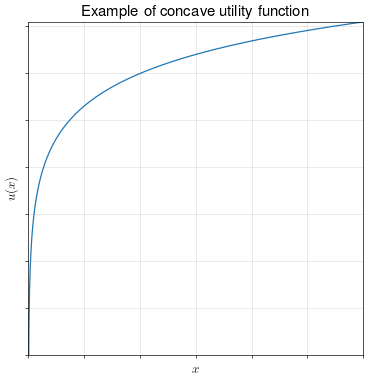
Definition. A function is concave if its second derivate is negative. That is, \(u^{\prime\prime}(x) < 0\) for all \(x\).
A concave function has a curvature which bends it towards zero, i.e. in an “inverse-U” shape:

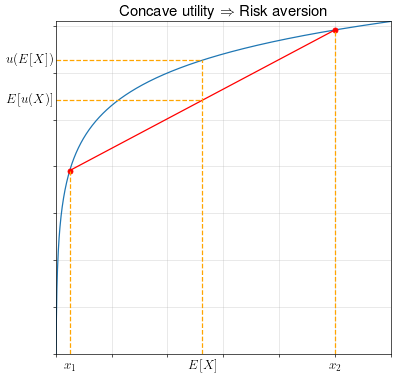
Theorem. If a person’s utility function \(u(X)\) over a random variable \(X\) is concave, then the person is risk averse.
Proof. We won’t do a full proof, but we can make an argument by looking at the diagram below.

In this example, \(X\) can take one of two values: \(x_1\) and \(x_2\). The point \((E[X], E[u(X)])\) will always lie on the red line, which is formed by the straight line between points \((x_1, u(x_1))\) and \((x_2, u(x_2))\).
Because of the concavity of the utility function, this straight line is always below the utility function. Thus, \(u(E[X])\) will always be above \(E[u(X)]\).
Example
Jack has an initial wealth of \(\$1,000\). There is a \(5\%\) chance he gets into a car accident, which would force him to pay \(\$200\) in repairs. Let \(X\) be a random variable representing Jack’s wealth at the end of the day. Jack’s utility function over wealth is \(u(X) = \sqrt{X}\).
Prove that Jack is risk averse by showing that his utility function is concave.
Answer.
\[\begin{align} u^\prime(x) &= \frac{1}{2} x^{-1/2} \\ u^{\prime \prime}(x) &= -\frac{1}{4} x^{-3/2} < 0 \end{align}\]The second derivative is negative for all \(x\). Therefore Jack is risk averse.
Economic Insight
People are risk averse if their utility function is concave. The greater the concavity of their utility function, the more risk averse they are.
It makes sense for peoples’ utility functions over wealth, income, and consumption to be concave. A concave utility function says that when your wealth is extremely low, even a little bit of additional wealth increases your utility by a lot. But if your wealth is already very high, a little bit of additional wealth will not increase your utility by much.
Certainty equivalence and insurance markets
Suppose a person faces an uncertain amount of wealth, \(X\). Their utility function over wealth is \(u(X)\). The certainty equivalent of \(X\), is defined as follows:
\[u(CE) = E[u(X)]\]That is, the certainty equivalent of a random wealth \(X\) is the amount of wealth that a person could have for certain that would give the same utility as the random wealth \(X\).
Certainty equivalent is a useful concept for calculating how much a person is willing to pay to avoid risk.
Example
Jack has an initial wealth of \(\$1,000\). There is a \(10\%\) chance he gets into a car accident, which would force him to pay \(\$200\) in repairs. Let \(X\) be a random variable representing Jack’s wealth at the end of the day. Jack’s utility function over wealth is \(u(X) = \ln{X}\).
Calculate Jack’s certainty equivalent of \(X\). How much is Jack willing to pay to avoid the risk of the car accident?
How much would it cost a risk neutral insurance company to insure Jack against his risk of a car accident?
Answer.
\[\begin{align} u(CE) &= E[u(X)] \\ \ln{CE} &= 0.9 \ln{1,000} + 0.1 \ln{800} = 6.8854 \\ CE &= e^{6.8854} = 977.93 \end{align}\]Jack would accept \(977.93\) wealth for certain versus having to face the uncertainty of \(X\).
Since his initial wealth is \(1,000\), this means that he’s willing to pay \(22.07\) to avoid the uncertainty of the car accident.
Since Jack has a \(10\%\) chance of incurring \(200\) in damages, a risk neutral insurance company could insure him at an expected cost of \(0.1 \times 200 = 20\). Thus, Jack is willing to pay more to avoid the risk than it would cost the insurance company to insure him.
Economic Insight
Risk averse people are willing to pay to reduce uncertainty. This opens up the market for insurance, where more risk averse individuals pay less risk averse organizations for insurance against uncertainty.