Exploring Utility Functions
In this lecture we explore the properties of various types of utility functions over two goods, \(u(x,y)\).
Cobb Douglas
A Cobb Douglas utility function has the following form:
\[u(x,y) = x^a y^b\]where \(a>0\) and \(b>0\).
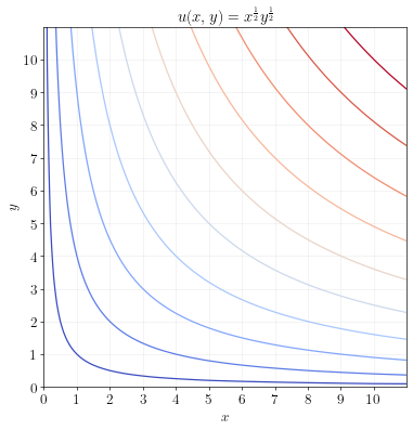
A Cobb Douglas utility function has indifference curves that look like:
The MRS between \(x\) and \(y\) in a Cobb Douglas utility function is:
\[MRS_{xy} (x,y) = \frac{u_x(x,y)}{u_y(x,y)} = \frac{ay}{bx}\]As can be seen from the MRS, Cobb Douglas has the realistic property of “taste for variety”. That is, the desirability of \(x\) relative to \(y\) goes down when the consumer consumes more of \(x\), and goes up when the consumer consumes more of \(y\).
Cobb Douglas also has the interesting property that the proportion of income a consumer spends on a good depends only on \(a\) and \(b\), and does not depend on the relative prices. (I leave it as an exercise for you to show this.)
Because of its flexibility and mathematical convenience, Cobb Douglas is a common choice for modeling consumer utility.
Cobb Douglas Example
A consumer derives utility over goods \(x\) and \(y\) given by:
\[u(x,y) = x^{\frac{2}{3}} y^{\frac{1}{3}}\]The consumer has income \(I=120\). The price of \(x\) is \(p_x = 20\) and the price of \(y\) is \(p_y = 10\).
Find the optimal choice of \(x\) and \(y\). Draw a diagram representing the consumer’s optimal choice.
Answer.
Step 1. Write down the optimization problem.
\[\max_{x,y} ~ x^{\frac{2}{3}} y^{\frac{1}{3}} ~ ~ \text{ s.t. } ~ ~ 20x + 10y = 120\]Step 2. Write down the first order conditions.
\[\begin{align} \tfrac{2}{3} x^{-\frac{1}{3}} y^{\frac{1}{3}} &= 20 \lambda \\ \tfrac{1}{3} x^{\frac{2}{3}} y^{-\frac{2}{3}} &= 10 \lambda \end{align}\]Step 3. Divide the two first order conditions.
\[\begin{align} \frac{\tfrac{2}{3} x^{-\frac{1}{3}} y^{\frac{1}{3}}}{\tfrac{1}{3} x^{\frac{2}{3}} y^{-\frac{2}{3}}} &= \frac{20\lambda}{10\lambda} \\ \frac{2y}{x} &= 2 \\ y&=x \end{align}\]Step 4. Plug \(y=x\) into the budget constraint.
\[\begin{align} 20x + 10y &= 120 \\ 20x + 10x &= 120 \\ 30x &= 120 \\ x &= 4 \end{align}\]Step 5. Use \(y=x\) to get \(y=4\).
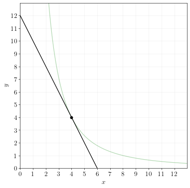
So the optimal choice is \(x=4\) and \(y=4\). The optimal choice is represented by the diagram below. (Instead of drawing many indifference curves, I’m only drawing the one that the optimal point lies on.)
Perfect Substitutes
If two goods \(x\) and \(y\) are perfect substitutes, then the utility function of the consumer must look like:
\[u(x,y) = ax + by\]where \(a>0\) and \(b>0\).
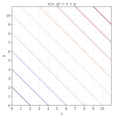
The indifference curves will be straight lines:
The MRS between \(x\) and \(y\) is:
\[MRS_{xy} (x,y) = \frac{u_x(x,y)}{u_y(x,y)} = \frac{a}{b}\]The MRS is constant, which means that the consumer is always willing to trade between \(x\) and \(y\) at a rate of \(a/b\). (The consumer is always willing to give up \(a/b\) units of \(y\) to get \(1\) unit of \(x\).)
Corner solutions
Perfect substitutes are interesting because the optimal choice is usually either a corner solution, or there are infinitely many optimal choices.
For example, consider your decision to choose between Exxon gasoline and Shell gasoline, which are perfect substitutes. If Exxon is cheaper, you would only purchase gas from Exxon and zero from Shell. On the other hand, if Shell is cheaper, you would only purchase from Shell and zero from Exxon. If they are the same price, then any combination of Shell and Exxon gasoline would be optimal.
Perfect Substitutes Example
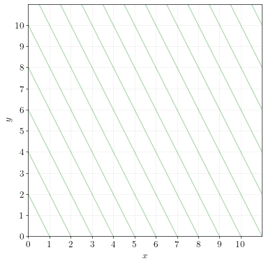
\(x\) and \(y\) are perfect substitutes. A consumer’s utility over \(x\) and \(y\) is represented by the indifference curves below.
The consumer has an income of \(80\). The price of \(x\) is \(p_x = 10\) and the price of \(y\) is \(p_y = 10\).
Plot the budget line and find the optimal choice of \(x\) and \(y\).
Answer.
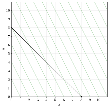
To plot the budget line, simply draw a straight line between the x and y intercepts. The x-intercept is \(I/p_x=8\) and the y-intercept is \(I/p_y=8\).
The optimal point is the point on the budget line that touches the highest indifference curve. That occurs at \(x=8\) and \(y=0\). Note that this is a corner solution.
Leontieff (Perfect Complements)
If two goods are perfect complements, we say that the consumer has a “Leontieff” utility function. A Leontieff utility function is defined by:
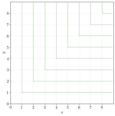
\[u(x,y) = \min (x,y)\]A Leontieff utility function has the following indifference curves:
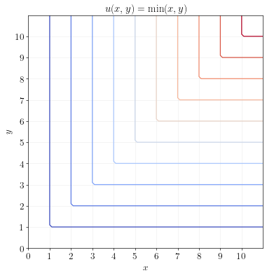
The MRS of a Leontieff utility function is tricky to define mathematically. It is either zero or infinity depending on the location.
Leontieff utility functions are used to model goods that require one another in order to be useful. For example, if \(x\) are left shoes and \(y\) are right shoes, then the utility over \(x\) and \(y\) is appropriately modeled by Leontieff utility.
The important thing to remember about Leontieff utility is that \(x\) and \(y\) must always be purchased in equal quantities.
Leontieff Example 1
\(x\) and \(y\) are perfect complements. A consumer’s utility over \(x\) and \(y\) is represented by the indifference curves below.
The consumer has an income of \(120\).
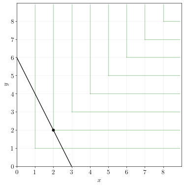
Plot the budget line and show the optimal choice when \(p_x = 40\) and \(p_y = 20\).
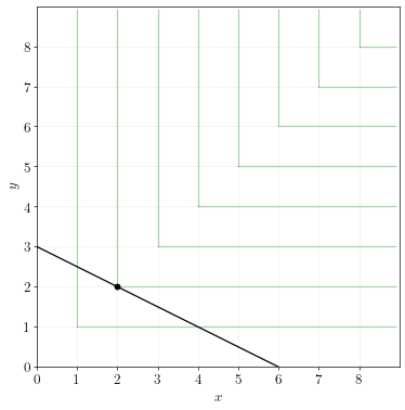
Plot the budget line and show the optimal choice when \(p_x = 20\) and \(p_y = 40\).
Answer.
The budget line when \(p_x=40\) and \(p_y=20\):
The budget line when \(p_x=20\) and \(p_y=40\):
In both cases, the optimal choice is \(x=2\) and \(y=2\).
Leontieff Example 2
Here is an alternative way to solve problems with Leontieff utility without drawing indifference curves.
A consumer’s utility over \(x\) and \(y\) is given by:
\[u(x,y) = \min (x, y)\]The consumer’s income is \(I=120\). The price of \(x\) is \(p_x=10\) and the price of \(y\) is \(p_y=20\). Calculate the optimal choice of \(x\) and \(y\).
Answer.
First note that at the optimal solution, \(x\) and \(y\) must be purchased in equal quantities. The total cost to buy both is \(p_x + p_y = 30\). Since the consumer’s income is \(I=120\), he can buy only \(I/(p_x+p_y) = 40\) pairs of \(x,y\). Thus, the optimal choice is \(x=40\) and \(y=40\).
Quasilinear Utility
A utility function is said to be quasilinear in \(x\) if it has the following form:
\[u(x,y) = x + v(y)\]You’ve already seen examples of quasilinear utility functions, which we worked with in lectures 4-8. In those examples, the utility function was quasilinear in the consumption of the “numeraire good” which we called \(c\) at the time.
Quasilinear utility functions have indifference curves are all parallel shifts along the \(x\) axis:
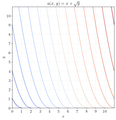
The MRS between \(y\) and \(x\) (that is, the amount of \(x\) the consumer is willing to give up for 1 unit of \(y\)) is:
\[MRS_{yx} (x,y) = \frac{u_y(x,y)}{u_x(x,y)} = v^\prime(y)\]If \(x\) is defined as numeraire consumption (e.g. money left over), then \(v^\prime(y)\) has an easy interpretation as the consumer’s marginal willingness-to-pay for good \(y\), as measured in dollar units.
Quasilinear utility functions are often used to model consumer choice between a single commodity and a generic measure of “money left over for other goods”.
Quasilinear Example
A consumer has quasilinear utility over \(x\) and \(y\):
\[u(x,y) = x + 20y^{\frac{1}{2}}\]The consumer’s income is \(I=100\). The price of \(x\) is \(p_x=1\) and the price of \(y\) is \(p_y = 2\).
Find the optimal choice of \(x\) and \(y\).
Answer.
Step 1. Write down the optimization problem.
\[\begin{align} \max_{x,y} ~ x + 20y^{\frac{1}{2}} ~ ~ \text{ s.t. } ~ ~ x + 2y = 100 \end{align}\]Step 2. Write down the first order conditions.
\[\begin{align} 1 &= \lambda \\ 10y^{-\frac{1}{2}} &= 2\lambda \end{align}\]Step 3. Plug \(\lambda=1\) into the first order condition for \(y\).
\[\begin{align} 10y^{-\frac{1}{2}} &= 2 \\ 5 &= y^{\frac{1}{2}} \\ 25 &= y \end{align}\]Step 4. Plug \(y=25\) into the budget constraint to get \(x\).
\[\begin{align} x + 2y &= 100 \\ x + 2(25) &= 100 \\ x + 50 &= 100 \\ x &= 50 \end{align}\]The optimal solution is \(x=50\) and \(y=25\).
