Constrained Multivariate Optimization
Setup
General problem
The general \(n\)-dimensional problem is:
\[\max_{x_1, \ldots, x_n} ~ f(x_1, \ldots, x_n) ~ \text{ s.t. } ~ g(x_1, \ldots, x_n) = 0\]That is, we want to find the values of \(x_1, \ldots, x_n\) that maximize \(f(x_1, \ldots, x_n)\), subject to the condition that \(g(x_1, \ldots, x_n) = 0\).
Note
We call \(f(x_1, \ldots, x_n)\) the objective function and we call \(g(x_1, \ldots, x_n)=0\) the constraint.
2-dimensional problem
For most of this class, we’ll only work with the two dimensional problem:
\[\max_{x,y} ~ f(x,y) ~ \text{ s.t. } ~ g(x,y) = 0\]That is, we want to find the values of \(x\) and \(y\) that maximize \(f(x,y)\), subject to the condition that \(g(x,y) = 0\).
Constrained optimization with contour maps
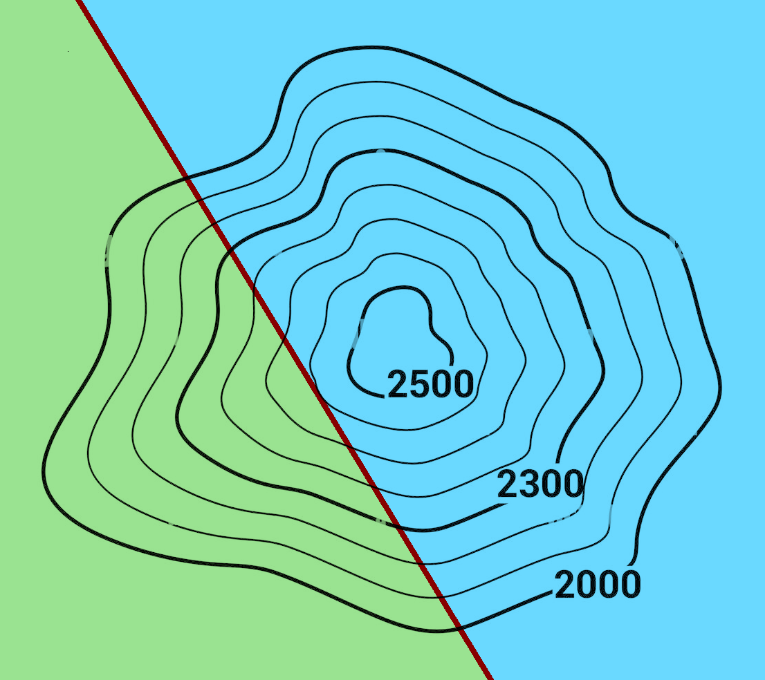
The image below shows the contour map of a mountain that spans the border of two countries. The border is marked by a red line. To the west of the border is Green Country, and to the east is Blue Country. What’s the highest point of the mountain that lies directly on the border?

This is an example of constrained optimization, because we’re looking for the highest point subject to the constraint that the point must lie on the border.
As it turns out, the maximum point lies on the contour which just touches the border, or constraint.
Mathematical Insight
In two dimensional constrained optimization, the maximal point is found on the contour line that just touches, i.e. is tangent to, the constraint.
Example 1
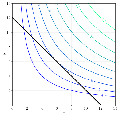
The diagram below shows contour lines for the function:
\[f(x,y) = x^{\frac{1}{2}} y^{\frac{1}{2}}\]The black line illustrates the constraint:
\[x + y = 12\]
Find the maximum of \(f(x,y)\) that lies on the constraint.
Answer. The maximum occurs at \(x=6, y=6\). The maximum value of the function is \(6\).
Constrained optimization with equations
General problem
For the general problem,
\[\max_{x_1, \ldots, x_n} ~ f(x_1, \ldots, x_n) ~ \text{ s.t. } ~ g(x_1,\ldots,x_n) = 0\]there are \(n\) first order conditions:
\[\frac{\partial}{\partial x_i} f(x_1, \ldots, x_n) = \lambda \frac{\partial}{\partial x_i} g(x_1, \ldots, x_n) ~ \text{ for each } ~ x_i\]There are \(n+1\) equations in \(n+1\) unknowns. The \(n+1\) unknowns are \(x_1, \ldots, x_n\) and \(\lambda\), which is called the Lagrange multiplier. The \(n+1\) equations are the \(n\) first order conditions and the constraint, \(g(x_1, \ldots, x_n)=0\).
Without delving too deep into the proof, the first order conditions essentially say that at the optimum, the partial derivative of the objective function is proportional to the partial derivative of the constraint. When the first order conditions hold, the constraint will be just touching the contour line of the objective function.
2-dimensional problem with linear constraint
In this class, we’ll mostly work with two-dimensional problems with linear constraints:
\[\max_{x, y} ~ f(x,y) ~ \text{ s.t. } ~ ax + by = c\]There are two first order conditions:
\[\begin{align} f_x(x,y) &= \lambda a \\ f_y(x,y) &= \lambda b \end{align}\]There are 3 equations in 3 unknowns. The unknowns are \(x\), \(y\), and \(\lambda\). The equations are the two first order conditions and the constraint, \(ax+bx+c=0\).
Example 2
Solve:
\[\max_{x,y} ~ xy ~ \text{ s.t. } ~ x + 2y = 12\]Answer using equations.
Step 1. Write down the first order condition for \(x\).
\[\begin{align} y = \lambda \end{align}\]Step 2. Write down the first order condition for \(y\).
\[\begin{align} x = 2\lambda \end{align}\]Step 3. Divide the two equations to get the relationship between \(x\) and \(y\):
\[\begin{align} \frac{x}{y} &= \frac{2\lambda}{\lambda} \\ \frac{x}{y} &= 2 \\ x &= 2y \end{align}\]Step 4. Plug this into the constraint to solve for \(y\).
\[\begin{align} x + 2y &= 12 \\ (2y) + 2y &= 12 \\ 4y &= 12 \\ y &= 3 \end{align}\]Step 5. Plug this back into the constraint to solve for \(x\).
\[\begin{align} x + 2y &= 12 \\ x + 2(3) &= 12 \\ x + 6 &= 12 \\ x &= 6 \end{align}\]The maximum value of \(xy\), subject to the constraint \(x+2y=12\), occurs at \(x=6\) and \(y=3\). The maximum value of the objective function is \(18\).
Answer using graphs.
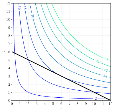
We could also have answered this question by plotting contour lines and the constraint.
The constraint can be plotted by re-arranging the constraint equation:
\[\begin{align} x + 2y &= 12 \\ 2y &= 12 - x \\ y &= 6 - \frac{1}{2}x \end{align}\]The contour line at elevation \(z\) can be plotted by re-arranging \(xy=z\):
\[\begin{align} xy &= z \\ y &= \frac{z}{x} \end{align}\]By plotting the constraint and the contour lines together, we get:
We can see that the maximum occurs at \(x=6\), \(y=3\), and \(z=18\).

