Theory of Consumer Choice
General setup
A consumer has income \(I\) and chooses how much of a good \(x\) and how much of a good \(y\) to consume.
The price of good \(x\) is \(p_x\) and the price of good \(y\) is \(p_y\). The consumer takes prices as given.
If the consumer purchases \(x\) units of good \(x\), and \(y\) units of good \(y\), he gets utility \(u(x,y)\).
The consumer’s optimization problem is:
\[\max_{x,y} ~ u(x,y) ~ \text{ s.t. } p_x x + p_y y = I\]We call \(u(x,y)\) the consumer’s utility function. It maps consumption onto a measure of the consumer’s total pleasure from consuming these goods. “Pleasure” is defined broadly, and it is assumed that consumers always try to maximize their utility.
We call the constraint, \(p_x x + p_y y = I\) the budget constraint. It basically says that the consumer can’t spend more than his income. (We also assume they spend all their income–we’ll deal with the possibility of borrowing and savings later.)
The consumer’s optimization problem is therefore to maximize their utility subject to their budget constraint.
First order conditions
This is a constrained multivariate optimization problem, which we can solve using the methods described in the previous chapters.
The first order conditions are:
\[\begin{align} u_x(x,y) &= \lambda p_x \\ u_y(x,y) &= \lambda p_y \end{align}\]This gives us three equations in three unknowns. The three unknowns are \(x\), \(y\), and \(\lambda\). The three equations are the two first order conditions and the budget constraint.
Marginal rate of substitution
If we divide the two first order condition equations by each other, we get:
\[\begin{align} \frac{u_x(x,y)}{u_y(x,y)} &= \frac{p_x}{p_y} \end{align}\]This says that at the optimal choice, the ratio of marginal utility of good \(x\) to the marginal utility of good \(y\) is equal to the ratio of prices.
We call the ratio of marginal utility between two goods the marginal rate of substitution between the two goods (or MRS).
At the consumer’s optimal choice, the marginal rate of substitution equals the ratio of the prices.
Intuitively, the marginal rate of substitution is the rate at which a consumer is willing to trade between the two goods. If the ratio of prices were not equal to the MRS, the consumer could improve their utility by purchasing less of one good and using the money saved to purchase more of the other. Thus, optimality requires that the MRS equals the ratio of prices.
Economic Insight
We call the ratio of marginal utility between two goods the marginal rate of substitution between the two goods.
At the consumer’s optimal choice between two goods, the marginal rate of substitution between those goods is equal to the ratio of prices.
Example
A consumer with income \(I = 50\) has a utility function over two goods, \(x\) and \(y\), given by:
\[u(x,y) = x^{\frac{1}{2}} y^{\frac{1}{2}}\]The price of good \(x\) is \(p_x = 2\) and the price of good \(y\) is \(p_y = 1\).
Calculate the consumer’s optimal choice of \(x\) and \(y\).
Answer.
Step 1. Write down the optimization problem.
\[\begin{align} \max_{x,y} ~ x^{\frac{1}{2}} y^{\frac{1}{2}} ~ \text{ s.t. } ~ 2x + y = 50 \end{align}\]Step 2. Write down the first order conditions:
\[\begin{align} \frac{1}{2} x^{-\frac{1}{2}} y^{\frac{1}{2}} &= 2 \lambda \\ \frac{1}{2} x^{\frac{1}{2}} y^{-\frac{1}{2}} &= 1 \lambda \end{align}\]Step 3. Divide the two first order conditions:
\[\begin{align} \frac{\frac{1}{2} x^{-\frac{1}{2}} y^{\frac{1}{2}}}{\frac{1}{2} x^{\frac{1}{2}} y^{-\frac{1}{2}}} &= 2 \\ \frac{y}{x} &= 2 \\ y &= 2x \end{align}\]Step 4. Plug \(y=2x\) into the budget constraint.
\[\begin{align} 2x + y &= 50 \\ 2x + (2x) &= 50 \\ 4x &= 50 \\ x &= 12.5 \end{align}\]Step 5. Plug \(x=12.5\) into the budget constraint to solve for \(y\).
\[\begin{align} 2x + y &= 50 \\ 2(12.5) + y &= 50 \\ 25 + y &= 50 \\ y &= 25 \end{align}\]So the consumer’s optimal choice is \(x=12.5\) and \(y=25\).
Graphical representation
The general consumer choice problem can be represented graphically as follows:
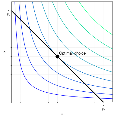
The budget constraint
The budget constraint will always be a straight line. The \(y\) intercept of the budget line is \(\frac{I}{p_y}\) (spend all the income \(y\)). The \(x\) intercept of the budget line is \(\frac{I}{p_x}\) (spend all income on \(x\)). The slope of the budget line is always \(-\frac{p_x}{p_y}\).
The indifference curves
The curves show the contour lines for the utility function. We also call these indifference curves because the consumer is indifferent between all the consumption bundles that lie on the same indifference curve.
Some features of indifference curves:
-
The utility is always increasing in the northeast direction. That’s \(x\) and \(y\) are assumed to be desirable goods, so more \(x\) and more \(y\) is always better.
- The degree of “bend” in the indifference curves is reflective of the consumer’s “taste for variety”, or the degree of substitutability between the two goods.
- If the indifference curves are very straight (low bend), then the consumer doesn’t care much about having variety between \(x\) and \(y\), i.e. the goods are highly substitutable.
- If the indifference curves are very curved (high bend), then the consumer cares a lot about having variety between \(x\) and \(y\), i.e. the goods are more complementary than substitutable.
- At any point \((x,y)\), the slope of the indifference curve at that point is: \(- \frac{u_x(x,y)}{u_y(x,y)}\). In other words, the slope of the indifference curves are equal the marginal rate of substitution between \(x\) and \(y\).
At the utility maximizing point, the budget line is just tangent to an indifference curve. Since the slope of the budget line is the ratio of \(p_x\) to \(p_y\), and the slope of the indifference curve is MRS, we see once again that utility is optimized when MRS equals the ratio of the prices.
Tip
To draw the graphical representation of consumer choice between two goods, make use of the following tidbits:
The slope of the budget line is always equal to \(- \frac{p_x}{p_y}\).
The y-intercept of the budget line is always \(\frac{I}{p_y}\).
The x-intercept of the budget line is always \(\frac{I}{p_x}\).
The utility-maximizing choice of \(x\) and \(y\) occurs on the indifference curve that is just tangent to (just touching) the budget line.
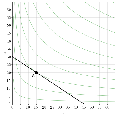
Graphical Example
A consumer with income \(I=90\) derives utility from two goods, \(x\) and \(y\). The price of \(x\) is \(p_x=2\) and the price of \(y\) is \(p_y=3\).
The consumer’s utility function is represented by the indifference curves shown in the diagram below.
Draw the budget line and find the optimal consumption of \(x\) and \(y\).
Answer.
To x-intercept of the budget line is \(I/p_x = 90/2 = 45\). The y-intercept of the budget line is \(I/p_y = 90/3 = 30\). The optimal point occurs on the indifference curve that just touches the budget line, which is marked by point “A” on the diagram below. The optimal consumption is \(x=15\) and \(y=20\).
Types of utility functions
We’ll now explore three types of utility functions, with different shapes for indifferent curves.
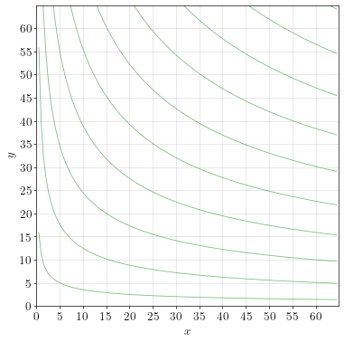
Cobb-Douglas utility
A Cobb Douglas utility function has the following form:
\[u(x,y) = x^a y^b\]where \(a>0\) and \(b>0\).
A Cobb Douglas utility function has indifference curves that look like:
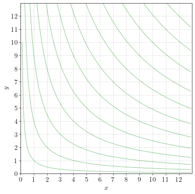
The MRS between \(x\) and \(y\) in a Cobb Douglas utility function is:
\[MRS_{xy} (x,y) = \frac{u_x(x,y)}{u_y(x,y)} = \frac{ay}{bx}\]As can be seen from the MRS, Cobb Douglas has the realistic property of “taste for variety”. That is, the desirability of \(x\) relative to \(y\) goes down when the consumer consumes more of \(x\), and goes up when the consumer consumes more of \(y\).
Cobb Douglas also has the interesting property that the proportion of income a consumer spends on a good depends only on \(a\) and \(b\), and does not depend on the relative prices. (I leave it as an exercise for you to show this.)
Because of its flexibility and mathematical convenience, Cobb Douglas is a common choice for modeling consumer utility.
Economic Insight
If a consumer has a Cobb Douglas utility function, the share of their budget they spend on each good depends only on the parameters of the utility function, and not on the relative prices of the goods.
Linear utility
A linear utility function has the following form:
\[u(x,y) = ax + by\]where \(a>0\) and \(b>0\).
The indifference curves will be straight lines:
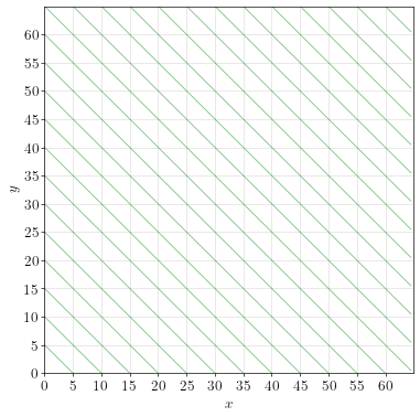
The MRS between \(x\) and \(y\) is:
\[MRS_{xy} (x,y) = \frac{u_x(x,y)}{u_y(x,y)} = \frac{a}{b}\]The MRS is constant, which means that the consumer is always willing to trade between \(x\) and \(y\) at a rate of \(a/b\). (The consumer is always willing to give up \(a/b\) units of \(y\) to get \(1\) unit of \(x\).)
Perfect substitutes
If a consumer has linear utility between two goods, then the two goods are perfect substitutes.
This also means that when deciding how much of \(x\) and \(y\) to buy, the consumer will usually only buy one or the other, but not both.
For example, consider your decision to choose between Exxon gasoline and Shell gasoline, which are perfect substitutes. If Exxon is cheaper, you would only purchase gas from Exxon and zero from Shell. On the other hand, if Shell is cheaper, you would only purchase from Shell and zero from Exxon.
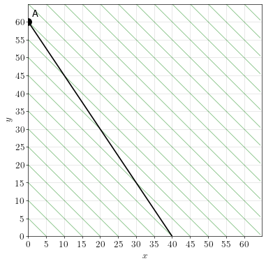
Linear Utility Example
A consumer’s utility over \(x\) and \(y\) is represented by the indifference curves below.
The consumer has an income of \(120\). The price of \(x\) is \(p_x = 3\) and the price of \(y\) is \(p_y = 2\).
Plot the budget line and find the optimal choice of \(x\) and \(y\).
Answer.
To plot the budget line, simply draw a straight line between the x and y intercepts. The x-intercept is \(I/p_x=40\) and the y-intercept is \(I/p_y=60\).
The optimal point is the point on the budget line that touches the highest indifference curve. That occurs at \(x=0\) and \(y=60\).
Leontieff utility
A Leontieff utility function has the following form:
\[u(x,y) = \min(x,y)\]The indifference curves will be right angles:
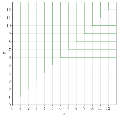
The MRS of a Leontieff utility function is tricky to define mathematically. It is either zero or infinity depending on the location.
Perfect complements
If a consumer has Leontieff utility between two goods, then the two goods are perfect complements.
Leontieff utility functions are used to model goods that require one another in order to be useful. For example, if \(x\) are left shoes and \(y\) are right shoes, then the utility over \(x\) and \(y\) is appropriately modeled by Leontieff utility.
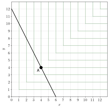
Leontieff Utility Example
A consumer’s utility over \(x\) and \(y\) is represented by the indifference curves below.
The consumer has an income of \(24\). The price of \(x\) is \(p_x = 4\) and the price of \(y\) is \(p_y = 2\).
Plot the budget line and find the optimal choice of \(x\) and \(y\).
Answer.
To plot the budget line, simply draw a straight line between the x and y intercepts. The x-intercept is \(I/p_x=6\) and the y-intercept is \(I/p_y=12\).
The optimal point is the point on the budget line that touches the highest indifference curve. That occurs at \(x=4\) and \(y=4\).