Unconstrained Multivariate Optimization
Setup
General problem
The general \(n\)-dimensional problem is:
\[\max_{x_1, \ldots, x_n} ~ f(x_1, \ldots, x_n)\]That is, we want to find the values of \(x_1, \ldots, x_n\) that maximize \(f(x_1, \ldots, x_n)\).
2-dimensional problem
For most of this class, we’ll focus our attention on the two dimensional problem:
\[\max_{x,y} ~ f(x,y)\]That is, we want to find the values of \(x\) and \(y\) that maximize \(f(x,y)\).
Contour maps
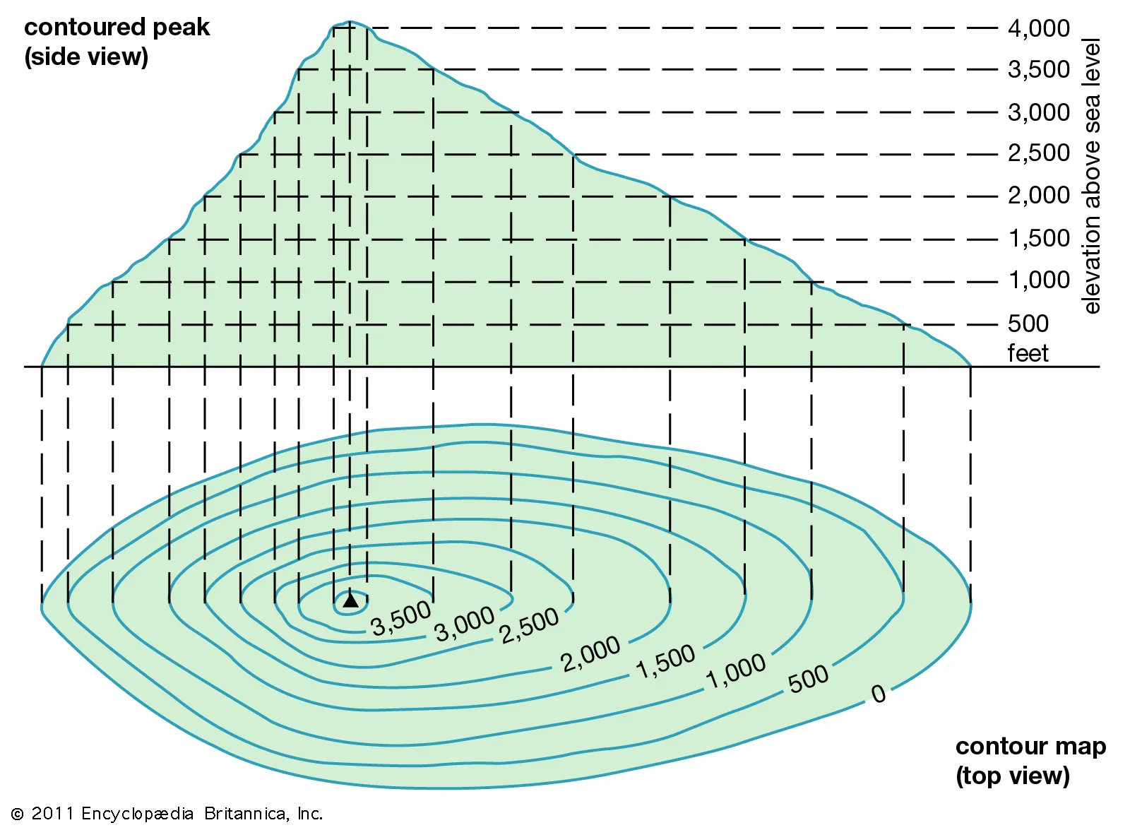
Here’s a picture of a mountain. What are the latitude and longitude coordinates of its peak?

One way to find the peak is to look at a contour map. A contour map shows lines of constant elevation:
Example 1
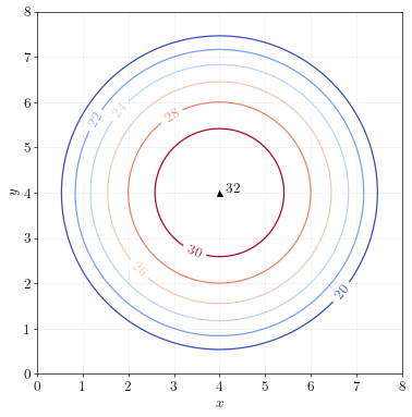
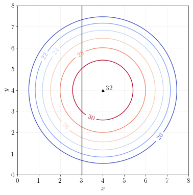
Look at the following two-dimensional function and its associated contour plot.
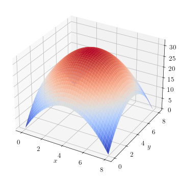
Find the \(x\) and \(y\) coordinates for the maximum of this function. What is the maximum?
Answer. The function is maximized at \(x=4\) and \(y=4\). The maximum is \(32\).
Plotting contour lines of functions
A contour line is a line of constant elevation, plotted on the \(x\) and \(y\) axes.
Suppose you have a function \(f(x,y)\). To find the contour line of the function at “elevation” equal to \(z\), you’d write down:
\[f(x,y) = z\]and then find all the combinations of \(x\) and \(y\) that give \(f(x,y)=z\).
Example 2
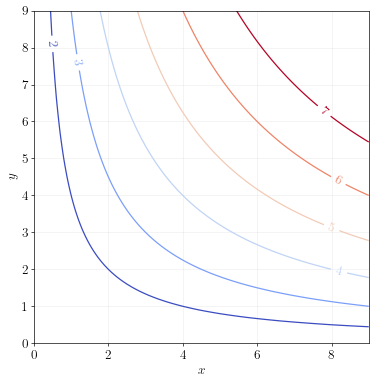
\[f(x,y) = x^{\frac{1}{2}} y^{\frac{1}{2}}\]Find the equation that describes the contour line for an elevation of \(z\). Then plot the contour lines for \(z=2, 3, 4, 5, 6,7\).
Answer.
To find the contour line at elevation \(z\), set \(f(x,y)=z\) and solve for \(y\):
\[\begin{align} x^{\frac{1}{2}} y^{\frac{1}{2}} &= z & \text{(definition of contour line)} \\ \left(x^{\frac{1}{2}} y^{\frac{1}{2}}\right)^2 &= z^2 & \text{(take both sides to the power of 2)} \\ xy &= z^2 & \text{(apply exponent rules)} \\ y &= \frac{z^2}{x} & \end{align}\]We can use this equation to plot the contour lines for various levels of \(z\), as shown below.
Partial derivatives
A partial derivative of a function shows the slope of the function when moving in a given direction.
Partial derivative with respect to x
Let’s call \(f_x(x,y)\) the partial derivative of \(f(x,y)\) with respect to \(x\). \(f_x(x,y)\) tells us the slope of \(f(x,y)\) when traveling in a straight line along the \(x\) direction, at a given level of \(y\).
Example 3
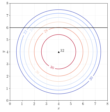
Imagine you are traveling from left to right along the black line (at \(y=6\)), shown below:
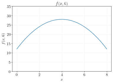
Your elevation at each level of \(x\) is like this:
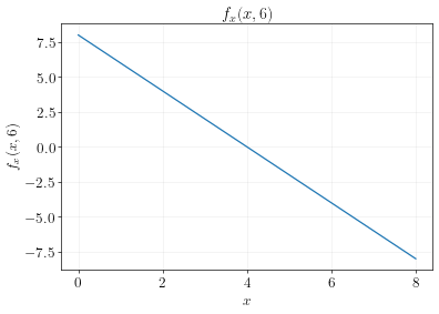
And the slope at each \(x\) for that particular slice of elevation is:
The partial derivative of \(f(x,y)\) with respect to \(x\) can be interpreted as the slope of the elevation sliced at a particular value of \(y\).
Notation Note
We’ll sometimes use the notation \(\frac{\partial}{\partial x} f(x,y)\) to describe the partial derivative of \(f(x,y)\) with respect to \(x\), instead of \(f_x(x,y)\).
Partial derivative with respect to \(y\)
Let’s call \(f_y(x,y)\) the partial derivative of \(f(x,y)\) with respect to \(y\). \(f_y(x,y)\) tells us the slope of \(f(x,y)\) when traveling in a straight line along the \(y\) direction, at a given level of \(x\).
Example 4
Imagine you are traveling from south to north along the black line (at \(x=3\)), shown below:
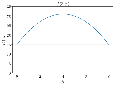
Your elevation at each level of \(y\) is like this:
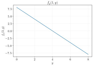
And the slope at each \(y\) for that particular slice of elevation is:
The partial derivative of \(f(x,y)\) with respect to \(y\) can be interpreted as the slope of the elevation sliced at a particular value of \(x\).
Notation Note
We’ll sometimes use the notation \(\frac{\partial}{\partial y} f(x,y)\) to describe the partial derivative of \(f(x,y)\) with respect to \(y\), instead of \(f_y(x,y)\).
Calculating the partial derivatives of a function
To calculate the partial derivative of a function with respect to \(x\), simply take the derivative of \(f(x,y)\) with respect to \(x\), treating \(y\) as a constant.
To calculate the partial derivative of a function with respect to \(y\), simply take the derivative of \(f(x,y)\) with respect to \(y\), treating \(x\) as a constant.
Example 5
\[f(x,y) = 8x - x^2 + 4y - y^3\]Calculate \(f_x(x,y)\) and \(f_y(x,y)\).
Answer.
\[\begin{align} f_x(x,y) &= 8 - 2x \\ f_y(x,y) &= 4 - 3y^2 \end{align}\]
Example 6
\[f(x,y) = x^{\frac{1}{2}} y^{\frac{1}{2}}\]Calculate \(f_x(x,y)\) and \(f_y(x,y)\).
Answer.
\[\begin{align} f_x (x,y) &= \frac{1}{2} x^{-\frac{1}{2}} y^{\frac{1}{2}} \\ f_y (x,y) &= \frac{1}{2} x^{\frac{1}{2}} y^{-\frac{1}{2}} \end{align}\]
Example 7
\[f(x,y) = x^2 \ln y\]Calculate \(f_x(x,y)\) and \(f_y(x,y)\).
Answer.
\[\begin{align} f_x (x,y) &= 2x \ln y \\ f_y (x,y) &= \frac{x^2}{y} \end{align}\]
First order conditions
In multivariate optimization, the maximum of a function is found at the point where the slope is zero in every direction. This means that all the partial derivatives are zero at the maximal point.
Mathematical Insight
In multivariate unconstrained optimization, the maximum of a function is found where partial derivatives are zero in every direction.
As in single variable optimization, we call the requirement that every partial derivative be zero the first order conditions.
General case
For the general case,
\[\max_{x_1, \ldots, x_n} ~ f(x_1, \ldots, x_n)\]there are \(n\) first order conditions:
\[\frac{\partial}{\partial x_i} f(x_1, \ldots, x_n) = 0 ~ ~ \text{ for each } ~ x_i\]That gives us \(n\) equations in \(n\) unknowns. (The unknowns are \(x_1, \ldots, x_n\).) If you’re interested in how to solve large systems of equations, you should take a math class called Linear Algebra.
2-dimensional case
For the 2-dimensional case:
\[\max_{x,y} ~ f(x,y)\]The first order conditions are:
\[\begin{align} f_x(x,y) &= 0 \\ f_y(x,y) &= 0 \end{align}\]Which is 2 equations in 2 unknowns (\(x\), \(y\)). Usually, it’s not too hard to solve systems of 2 equations in 2 unknowns. In fact, you’ve been solving systems of up to 4 equations in 4 unknowns already!
Example 8
\[f(x,y) = 12x + xy - 0.5x^2 - y^2\]Find the maximum of \(f(x,y)\).
Answer.
Step 1. Write down the partial derivatives.
\[\begin{align} f_x(x,y) &= 12 + y - x \\ f_y(x,y) &= x - 2y \end{align}\]Step 2. Write down the first order conditions.
\[\begin{align} 12 + y - x &= 0 \\ x - 2y &= 0 \end{align}\]Step 3. Solve the first order conditions.
We’ll work by first writing \(x\) in terms of \(y\), using the second equation, then substituting that into the first equation.
\[\begin{align} x &= 2y & \text{(rearrange the FOC for y)} \\ 12 + y - (2y) &= 0 & \text{(substitute } x=2y \text{ into the FOC for x} 12 - y &= 0 \\ y &= 12 & \\ x &= 2(12) = 24 & \end{align}\]So \(f(x,y)\) is maximized at \(x=24\) and \(y=12\). To get the value of \(f(x,y)\) at the maximum, simply plug these numbers into the function.
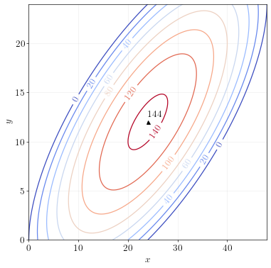
\[\begin{align} f(24,12) &= 12x + xy - 0.5x^2 - y^2 \\ &= 12(24) + (24)(12) - 0.5(24)^2 - (12)^2 \\ &= 144 \end{align}\]So the maximum value of \(f(x,y)\) is \(144\).
If you were to graph the contour lines of this function, you’d get:
