Application: Productivity Shocks

• Graphical Analysis
  • First order effects
  • Second order effects
  • Third order effects… ?
• General Solution of a Mathematical Model
• Solution for a Class of Models
  • Setup
  • Solution
    • Consumer’s problem
    • Worker’s problem
    • Firm’s problem
    • Solution
  • Discussion

In this lecture, we’ll explore what happens when there’s a technological shock that boosts the firm’s productivity.

Suppose a new technology is invented that increases the marginal productivity of workers. That is, a single worker can now produce more output with a single hour of work than they could before. This means that the firm can produce more output with the same amount of labor. Equivalently, it means that the firm can produce the same amount of output with less labor. What does it do to equilibrium wage rates and commodity prices?

Humans have wrestled with these questions for generations. It seems that every time a new technology is invented, people worry about what impact that will have on the labor market and the economy.

(Quote about working fewer hours). Nowadays, the question on everyone’s mind is what Generative Artificial Intelligence will do to the labor market.

Today’s lecture will help us think about these issues rigorously.

Graphical Analysis

First order effects

Let’s first approach the question using supply and demand diagrams, as we would in a first-year microeconomic theory course.

Since we’re interested in both wages and commodity prices, we need to draw supply and demand diagrams for both the commodity market and the labor market.

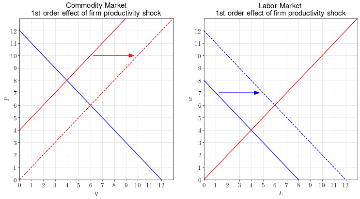
In the commodity market, the increase in firm productivity should reduce the marginal cost of production. This is reflected by an outward shift in the commodity supply curve.

In the labor market, the increase in firm productivity should increase labor demand. (Since the marginal productivity of a worker has increased, the firm is willing to pay more for each worker.) This is reflected by an outward shift in the labor demand curve.

Based on these effects, we’d predict an increase in the equilibrium wage and a decrease in the equilibrium commodity price.

Second order effects

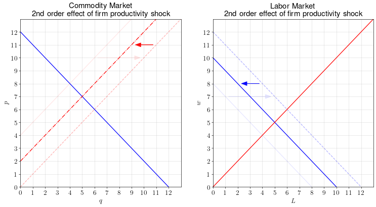
But we can’t end the analysis there. The problem is that when the wage increases, the firm’s marginal costs go up, which would shift the supply curve left. And when the commodity price decreases, the firm’s marginal revenue product of labor goes down, which would shift the labor demand curve left.

We call these “second order effects” because they happen as a response to the price changes induced by the first order effects.

These second order effects run counter to the first order effects.

Third order effects… ?

But the second order effects would cause third order effects, and so on. When does the chain of events end and the markets settle on a new equilibrium?

Unfortunately, we can’t answer those questions using just the supply and demand diagrams. Answering this question requires us to write down a mathematical model of the players in the economy: namely, the consumers, workers, and firms.

Economic Insight

A productivity shock seems to lead to an endless chain of events affecting both the commodity market and the labor market. We won’t be able to make a precise prediction without specifying a mathematical model.

General Solution of a Mathematical Model

To model a technological productivity shock, we write the firm’s production function as \(A f(L)\). The productivity shock itself is modeled as an increase in \(A\). (That is, for the same labor input, more commodity output can be produced.)

The equilibrium conditions are the same as from lecture 6, just with the inclusion of \(A\) wherever \(f(L)\) or \(f^\prime(L)\) used to be:

\[\begin{align} p &= v^\prime(q_d) ~ ~ ~ ~ & (\text{Eq.1}) \\ w &= d^\prime(L_s) ~ ~ ~ ~ & (\text{Eq.2}) \\ w &= p A f^\prime(L_d) ~ ~ ~ ~ & (\text{Eq.3}) \\ q_d &= q_s = q ~ ~ ~ ~ & (\text{Eq.4}) \\ L_d &= L_s = L ~ ~ ~ ~ & (\text{Eq.5}) \\ q &= Af(L) ~ ~ ~ ~ & (\text{Eq.6}) \end{align}\]

Solving this system of 6 equations in 6 unknowns would tell us the equilibrium outcome as a function of \(A\).

Ultimately, the equilibrium of the model depends on the “exogenous” features of the model, which are also called the “model primitives”:

• The consumer’s benefit function over the commodity: \(v(q)\)
• The worker’s disutility of labor: \(d(L)\)
• The firm’s production function: \(Af(L)\)

Solution for a Class of Models

Let’s now work out a general solution for a specific class of models, in which we assume certain funtional forms for \(v(q)\), \(d(L)\), and \(Af(L)\).

Setup

A representative, price-taking consumer decides how many units, \(q\), of a commodity to purchase at unit price \(p\). The utility they receive for purchasing \(q\) units at price \(p\) is:

\[u(q) = \alpha \ln q - pq\]

A representative, price-taking worker decides how many units, \(L\), of labor to supply at unit wage \(w\). The worker’s utility function over working \(L\) labor-units at wage \(w\) is:

\[u(L) = wL - \frac{1}{2} \delta L^2\]

A representative, price-taking firm uses labor to produce and sell a commodity at unit price \(p\). The firm hires labor at a constant wage rate \(w\). If the firm employs \(L\) units of labor, it can produce \(f(L)\) units of commodity output, where:

\[f(L) = AL^{1/2}\]

In this setup:

• \(\alpha\) controls how much the consumers like the commodity
• \(\delta\) controls how much the workers dislike work
• \(A\) controls the firm’s productivity

We will derive expressions for the equilibrium wage and commodity price in terms of \(A\), \(\delta\), and \(\alpha\).

Solution

Consumer’s problem

The consumer’s first order condition is:

\[\frac{\alpha}{q} - p = 0\]

which gives us the inverse commodity demand curve:

\[p = \frac{\alpha}{q} ~ ~ ~ ~ \text{(Eq.1)}\]

Worker’s problem

The worker’s first order condition is:

\[w - \delta L = 0\]

which gives us the inverse labor supply function:

\[w = \delta L ~ ~ ~ ~ \text{(Eq.2)}\]

Firm’s problem

The firm’s optimization problem is:

\[\max_{L} ~ pAL^{1/2} - wL\]

which leads to the first order condition:

\[\frac{1}{2} pA L^{-1/2} - w = 0\]

and the inverse labor demand function:

\[w = \frac{1}{2} pA L^{-1/2} ~ ~ ~ ~ \text{(Eq.3)}\]

Solution

To find the solution, we follow the following steps:

Step 1. Use Eq.1 and Eq.2 to plug in for \(p\) and \(w\) in Eq.3, and rearrange to put \(q\) and \(L\) on the same side:

\[\begin{aligned} w &= \frac{1}{2} pAL^{-1/2} ~ ~ ~ ~ & \text{(Eq.3)} \\ \delta L &= \frac{1}{2} \left(\frac{\alpha}{q}\right) AL^{-1/2} ~ ~ ~ ~ & \text{(Plug in Eq.1 and Eq.2)} \\ \delta L L^{1/2} &= \frac{1}{2} \left(\frac{\alpha}{q}\right) A ~ ~ ~ ~ & \text{(Multiply both sides by }L^{1/2}\text{)} \\ \delta L^{3/2} &= \frac{1}{2} \left(\frac{\alpha}{q}\right) A ~ ~ ~ ~ & \\ \delta q L^{3/2} &= \frac{1}{2} \alpha A ~ ~ ~ ~ & \text{(Divide both sides by q)} \\ qL^{3/2} &= \frac{\alpha A}{2\delta} ~ ~ ~ ~ & \text{(Divide both sides by }\delta\text{)} \end{aligned}\]

Step 2. Plug \(q = AL^{1/2}\) into the previous equation and rearrange to solve for \(L\).

\[\begin{aligned} qL^{3/2} &= \frac{\alpha A}{2\delta} ~ ~ ~ ~ & \\ AL^{1/2} L^{3/2} &= \frac{\alpha A}{2 \delta} ~ ~ ~ ~ & \text{(Plug in }q=AL^{1/2}\text{)} \\ A L^{2} &= \frac{\alpha A}{2 \delta} ~ ~ ~ ~ & \\ L^{2} &= \frac{\alpha}{2 \delta} ~ ~ ~ ~ & \text{(Divide both sides by A)} \\ L &= \sqrt{\frac{\alpha}{2\delta}} ~ ~ ~ ~ & \text{(Eq.L)} \end{aligned}\]

Plugging this formula for \(L\) into Eq.2, we get:

\[\begin{aligned} w &= \delta \sqrt{\frac{\alpha}{2 \delta}} ~ ~ ~ ~ & \\ w &= \sqrt{\frac{\alpha \delta}{2}} ~ ~ ~ ~ & \text{(Eq.w)} \end{aligned}\]

Using \(q = AL^{1/2}\), we get:

\[\begin{aligned} q &= AL^{1/2} ~ ~ ~ ~ & \\ q &= A\left(\sqrt{\frac{\alpha}{2 \delta}}\right)^{1/2} ~ ~ ~ ~ & \\ q &= A \left(\frac{\alpha}{2 \delta}\right)^{1/4} ~ ~ ~ ~ & \text{(Eq.q)} \end{aligned}\]

Lastly, we take this formula for \(q\) and plug it into Eq.1 to get \(p\):

\[\begin{aligned} p &= \frac{\alpha}{q} ~ ~ ~ ~ & \\ p &= \frac{\alpha}{A \left( \frac{\alpha}{2\delta} \right)^{1/4} } ~ ~ ~ ~ & \\ p &= \frac{\alpha}{A} \left(\frac{\alpha}{2\delta}\right)^{-1/4} ~ ~ ~ ~ & \\ p &= \frac{\alpha^{3/4} (2\delta)^{1/4}}{A} ~ ~ ~ ~ & (\text{Eq.p}) \end{aligned}\]

Discussion

We discovered that in equilibrium:

\[\begin{aligned} L &= \sqrt{\frac{\alpha}{2\delta}} \\ w &= \sqrt{\frac{\alpha \delta}{2}} \\ q &= A \left(\frac{\alpha}{2 \delta}\right)^{1/4} \\ p &= \frac{\alpha^{3/4} (2\delta)^{1/4}}{A} \end{aligned}\]

Using these equations, we can discuss how the equilibrium changes when \(\alpha\), \(\delta\), or \(A\) change.

• If \(\alpha\) increases (the consumer’s desire for the commodity increases):
  • The equilibrium quantity of labor increases
  • The equilibrium wage rate increases
  • The equilibrium quantity of commodity increases
  • The equilibrium commodity price increases
• If \(\delta\) increases (the worker’s disutility for labor increases):
  • The equilibrium quantity of labor decreases
  • The equilibrium wage rate increases
  • The equilibrium quantity of commodity decreases
  • The equilibrium commodity price increases
• If \(A\) increases (the firm’s productivity increases):
  • The equilibrium quantity of labor stays the same
  • The equilibrium wage rate stays the same
  • The equilibrium quantity of commodity increases
  • The equilibrium commodity price decreases

Our analysis therefore shows that, for this class of models, a technological shock that increases productivity has no long run effect on the labor market. Rather, the benefits to the technology are entirely experienced by the consumers of the commodity market, who can buy more of the commodity at lower price.

Economic Insight

Under certain conditions, it’s possible for a productivity shock to have no long run effects on equilibrium wage rate or employment levels. Instead, the impact is felt primarily in the commodity market, through lower prices and higher quantities. The main beneficiary of the technological shock is therefore the commodity consumers.

This insight can explain why productivity shocks have not historically led to people working less while consuming the same amount, but rather it has led to people working about the same amount, but consuming more.

Economic Insight

Mathematical models help us understand how the economy will respond to specific events. The models help in the following ways:

1. The models can tell us what parameters are are important in determining the outcome (e.g. disutility of labor, utility of consumption, etc.)

2. Knowing which parameters are important helps guide our research into what data we need to collect and analyze to estimate these parameters.

3. If we have estimates of the model parameters, the model lets us make more precise, quantitative predictions about outcomes.