Demand Curves
- General setup
- Quasilinear utility
- Demand curves
- Consumer surplus
- Price and marginal willingness-to-pay
General setup
Let there be a commodity with price \(p\), which consumers take as given.
A consumer with income \(Y\) gets utility from consuming this commodity. If the consumer consumes \(q\) units of the commodity, then they have \(c = Y-pq\) dollars left to spend on other goods.
The consumer gets utility from consumption of the commodity \(q\) and consumption of other goods \(c\). They choose \(c\) and \(q\) to maximize their utility, \(u(c,q)\).
The optimization problem the consumer solves is:
\[\max_{c,q} ~ u(c,q) ~ ~ \text{ s.t. } ~ ~ c = Y - pq\]Note 1
We’ll sometimes call \(c\) the numeraire good, because it is the unit of account by which all other goods are evaluated.
Note 2
\(c = Y - pq\) is called the budget constraint because it says that the consumer cannot spend more than their income.
Quasilinear utility
Today, we’ll focus on solving the consumer optimization problem for a special class of utility functions known as quasilinear utility functions. These utility functions have the form:
\[u(c,q) = c + v(q)\]That is, utility increases linearly in the numeraire good \(c\), but can increase arbitrarily with the commodity \(q\).
Example 1
The consumer’s utility function over numeraire consumption \(c\) and commodity consumption \(q\) is:
\[u(c,q) = c + 10q - 0.5q^2\]The price of the commodity is \(p=5\), and the consumer’s income is \(Y=100\).
- How many units of the commodity will the consumer purchase?
- How much money will they spend on the commodity?
- How much money will they have left over?
- What is their utility at the optimal choice?
Answer.
First, set up the optimization problem:
\[\max_{c,q} ~ c + 10q - 0.5q^2 ~ ~ \text{ s.t. } ~ ~ c = 100 - 5q\]Plug \(c = 100 - 5q\) into \(c\) in the objective function:
\[\begin{align} & \max_{q} ~ 100 - 5q + 10q - 0.5q^2 \\ = & \max_{q} ~ 100 + 5q - 0.5q^2 \end{align}\]The objective function is now \(100 + 5q - 0.5q^2\). To find the \(q\) that maximizes this, we simply need to solve the first order condition:
\[\begin{aligned} \frac{d}{dx} (100 + 5q - 0.5q^2) &= 0 & \text{(this is the first order condition)} \\ 5 - q &=0 & \text{(apply derivative rules)} \\ 5 &= q & \text{(add q to both sides)} \end{aligned}\]So here are our answers:
\[\begin{align} u(c,q) &= c + 10q - 0.5q^2 \\ &= 75 + 10(5) - 0.5(5)^2 \\ &= 112.5 \end{align}\]
- The consumer will purchase \(q=5\) units of the commodity.
- The consumer spends \(pq = 25\) dollars on the commodity.
- The consumer has \(c = Y - pq = 75\) dollars left over.
- The consumer’s utility at this choice is:
Demand curves
A demand curve maps the price of a commodity to the quantity that a consumer buys. We can solve the opimization problem for a general price \(p\) to get the consumer’s demand curve.
Example 2
The consumer’s utility function over numeraire consumption \(c\) and commodity consumption \(q\) is:
\[u(c,q) = c + 10q - 0.5q^2\]The price of the commodity is \(p\), and the consumer’s income is \(Y=100\).
Calculate how many units of the commodity the consumer will purchase, expressed as a function of the price \(p\).
Answer.
Write down the consumer’s optimization problem:
\[\max_{q} ~ 100 - pq + 10q - 0.5q^2\]Solve the first order condition:
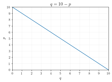
\[\begin{align} \frac{d}{dx} (100 -pq + 10q - 0.5q^2) &= 0 & \text{(first order condition)} \\ -p + 10 - q &= 0 & \text{(apply derivative rules)} \\ 10 - p &= q & \text{(add q to both sides)} \end{align}\]Thus, it is optimal to choose \(q = 10 - p\). This is the demand curve, because it maps \(p\) to the optimal choice of \(q\).
The graph of the demand curve is plotted below.
Consumer surplus
Consumer surplus is the gain in utility that a consumer gets from consuming \(q\) units of the commodity vs. consuming 0. We can calculate consumer surplus using graphs or using equations.
The advantage of calculating consumer surplus using equations is that it works for any type of demand curve, even if the demand curve isn’t a straight line.
Example 3
The consumer’s utility function over numeraire consumption \(c\) and commodity consumption \(q\) is:
\[u(c,q) = c + 10q - 0.5q^2\]The price of the commodity is \(p\), and the consumer’s income is \(Y=100\). Calculate consumer surplus when the price of the commodity is \(p=5\).
Answer using graphs.
For this problem, we already derived the demand curve. The demand curve was: \(q = 10 - p\).
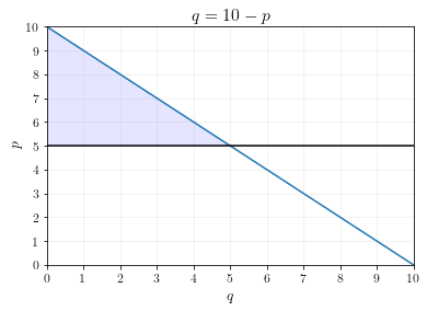
In Econ 160, you learned how to calculate consumer surplus using graphs. The consumer surplus at \(p=5\) is the shaded triangle underneath the demand curve and above the price, as shown below.
The area of this triangle is \(\frac{1}{2} (5)(5) = 12.5\), so consumer surplus is \(12.5\).
Answer using equations.
For this problem, we already saw that the consumer’s total utility when \(p=5\) was \(112.5\). This is not the same as consumer surplus, however, because you have to compare this utility to the utility from buying \(q=0\).
If the consumer buys \(q=0\), then their numeraire consumption is \(c=100\). Their utility is:
\[\begin{align} u(c,q) &= c + 10q - 0.5q^2 \\ &= 100 + 10(0) + 0.5(0)^2 \\ &=100 \end{align}\]So the consumer gets \(100\) utility if they consume \(q=0\), and \(112.5\) utility if they consume \(q=5\) at a price of \(p=5\). Thus, the consumer surplus is \(112.5 - 100 = 12.5\), which it the same as what we calculated using the graph.
Example 4
In this example, we’ll be forced to calculate consumer surplus using equations.
The consumer’s utility function over numeraire consumption \(c\) and commodity \(q\) is:
\[u(c,q) = c + 24q^{0.5}\]The consumer’s income is \(Y=50\). Calculate consumer surplus if the price of the commodity is \(p=4\).
Answer.
Set up the optimization problem:
\[\max_{q} ~ 50 - pq + 24q^{0.5}\]Solve the first order conditions:
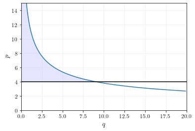
\[\begin{align} -p + 12q^{-0.5} &= 0 \\ 12q^{-0.5} &= p \\ q^{-0.5} &= \frac{p}{12} \\ q &= \left(\frac{p}{12}\right)^{-2} \end{align}\]If we were to plot this function and calculate the consumer surplus at \(p=4\), we’d get the following graph.
The shaded area is not a triangle, so we can’t calculate the area using a simple geometric formula.
Instead, let’s calculate consumer surplus using the utility equation. At \(p=4\), we calculate \(q=9\) and \(c=14\). Utility is \(86\). If \(q=0\), then \(c=50\) and utility is \(50\). The consumer surplus at \(p=4\) is therefore \(86-50=36\).
Price and marginal willingness-to-pay
Let’s return to the general setup with quasilinear utility:
\[\max_{c,q} ~ c + v(q) ~ ~ \text{ s.t. } ~ ~ c = Y - pq\]Which we can rewrite as:
\[\max_{q} ~ Y - pq + v(q)\]The first order condition for this optimization problem is:
\[-p + v^\prime(q) = 0\]So at the optimal choice of \(q\), the following equation holds:
\[p = v^\prime(q)\]In other words, at the optimal choice of \(q\), price equals the marginal utility that the consumer gets from consumption of \(q\).
In the quasilinear framework, utility has a 1:1 relationship with dollars spent on the numeraire good. Thus, marginal utility equals marginal willingness to pay.
Thus, in the equilibrium of any market where consumers are price-takers, they will consume up to the quantity where price equals their marginal willingness to pay.
Economic Insight
In the equilibrium of a market where consumers are price takers, price equals consumers’ marginal willingness to pay.
This is a useful insight, because it means that price is a good measure of how much value consumers derive from their consumption of a commodity. Higher priced goods are valued more highly by the marginal consumer than lower priced goods.


