Supply Curves
General setup
A firm produces a commodity which it can sell at price \(p\). The firm takes the price as given.
The firm’s total cost to produce \(q\) units of the commodity is \(c(q)\).
If the firm produces \(q\) units of the commodity, it gets revenue equal to \(pq\) and it pays a total cost of \(c(q)\). The firm’s profit function \(\Pi(q)\), which maps quantity of output to profit, is therefore:
\[\Pi(q) = pq - c(q) ~ ~ ~ ~ \text{(Profit = Revenue - Cost)}\]The firm’s goal is to choose its output level, \(q\), to maximize profit:
\[\max_{q} ~ \Pi(q)\]Note
In optimization theory, we call the function we’re trying to maximize the objective function.
First order condition
Profit is maximized when the derivative of the profit function is equal to zero.
\[\begin{align} \Pi^\prime(q) &= 0 & \text{(first order condition)} \\ \frac{d}{dq} \left[ pq - c(q) \right] &= 0 & \\ p - c^\prime(q) &= 0 & \text{(apply derivative rules)} \\ p &= c^\prime(q) & \text{(add } c^\prime(q) \text{ to both sides)} \end{align}\]Thus, at the firm’s optimal choice of \(q\), price equals marginal cost.
Note
The marginal cost at \(q\) is the slope of the cost function at \(q\), thus: marginal cost at \(q\) is the derivative of the cost function at \(q\).
Economic Insight
In the equilibrium of a market where firms are price takers, price equals the firms’ marginal cost of production.
Example 1
The price of a commodity is \(p=10\). A firm can produce \(q\) units of the commodity at a total cost of:
\[c(q) = q^2\]What choice of \(q\) maximizes the firm’s total profit? What is the maximum profit the firm could achieve?
Answer.
The firm’s profit function is:
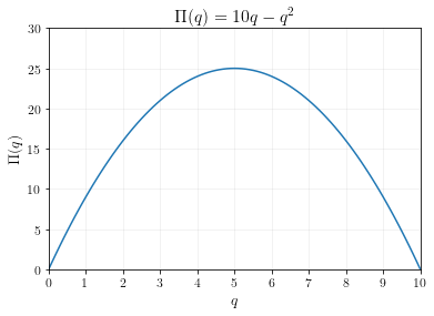
\[\begin{align} \Pi(q) &= pq - c(q) \\ &= 10q - q^2 \end{align}\]If we were to plot the profit function, it would look like this:
To find the maximum of the profit function, we solve the first order condition:
\[\begin{align} \Pi^\prime(q) &= 0 & \text{(first order condition)} \\ \frac{d}{dq} \left[ 10q - q^2 \right] &= 0 & \\ 10 - 2q &=0 & \text{(apply derivative rules)} \\ 10 &= 2q & \text{(add 2q to both sides)} \\ 5 &= q & \text{(divide both sides by 2)} \end{align}\]Thus, profit is maximized by producing \(q=5\) units of output.
To calculate the actual profit, simply plug \(q=5\) back into the profit function:
\[\begin{align} \Pi(5) = 10(5) - (5)^2 = 50 - 25 = 25 \end{align}\]So the maximum profit the firm could achieve is \(25\).
Supply curves
A supply curve maps the price of a commodity to the amount of output a producer chooses to produce. We can solve the optimization problem for a general price \(p\) to get the producer’s supply curve.
Example 2
The price of a commodity is \(p\). A firm can produce \(q\) units of the commodity at a total cost of:
\[c(q) = q^2\]Calculate how many units of the commodity the producer will produce, expressed as a function of the price \(p\).
Answer.
The firm maximizes:
\[\max_{q} ~ pq - q^2\]The first order condition is:
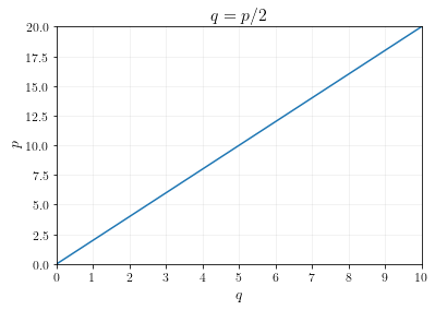
\[\begin{align} \frac{d}{dq} \left[ pq - q^2 \right] &= 0 \\ p - 2q &= 0 \\ p &= 2q \\ \frac{p}{2} &= q \end{align}\]When price is \(p\), the optimal quantity of output is \(q = p/2\). This is the supply curve.
The graph of this supply curve is plotted below.
Producer surplus
Producer surplus is the gain in profit that a producer gets from producing \(q\) units of output vs. producing 0. (In other words, it is equal to the variable profit.) We can calculate producer surplus using graphs or using equations.
The advantage of calculating producer surplus using equations is that it works for any kind of supply curve, even if the supply curve isn’t a straight line.
Example 3
The price of a commodity is \(p\). A firm can produce \(q\) units of the commodity at a total cost of:
\[c(q) = q^2\]Calculate producer surplus when the price of the commodity is \(p=10\).
Answer using graphs.
For this problem, we already derived the supply curve. It was \(q = p/2\).
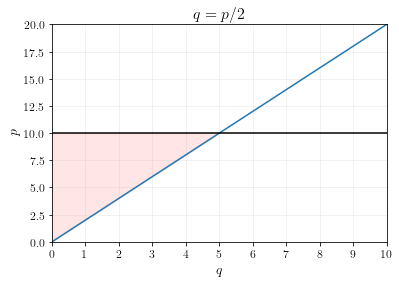
In Econ 160, you learned how to calculate producer surplus using graphs. The producer surplus at \(p=10\) is the shaded triangle underneath the price and above the supply curve, as shown below.
The area of the triangle is \(\frac{1}{2}(5)(10) = 25\), so the producer surplus is \(25\).
Answer using equations.
When price is \(p=10\), the firm will produce \(q=5\) units of output. Plugging that into the profit equation, \(\Pi(q) = 10q - q^2\) gives a profit of \(25\), which is same as the answer we got graphically.
Example 4
In this example, we’ll be forced to calculate producer surplus using equations.
Let the producer’s cost function be:
\[c(q) = q^3\]Calculate the producer surplus if the price of the commodity is \(p=5\).
Answer.
The firm’s optimization problem is:
\[\max_{q} ~ pq - q^3\]Solve the first order conditions:
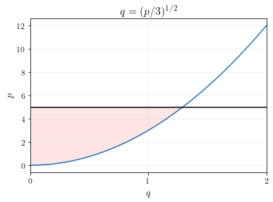
\[\begin{align} p - 3q^2 &= 0 & \text{(first order condition)} \\ p &= 3q^2 & \text{(add } 3q^2 \text{ to both sides)} \\ \frac{p}{3} &= q^2 & \text{(divide both sides by 3)}\\ \left(\frac{p}{3}\right)^{1/2} &= q & \text{(inverse rule for exponents)} \end{align}\]If we were to plot this supply curve and calculate the producer surplus at \(p=5\), we’d get the following graph.
The shaded area is not a triangle, so we can’t calculate the area using a simple geometric formula.
Instead, let’s calculate the producer surplus using equations. At \(p=5\), the optimal choice of output is \(q=(5/3)^{1/2}=1.29\). Profit at \(q=1.29\) is equal to \(\Pi(1.29) = (5)(1.29) - (1.29)^3 = 4.30\).
Since profit is \(0\) when \(q=0\) (there is no fixed cost), the producer surplus is \(4.30\).


