Single Variable Optimization
- Graphical intuition
- Slopes of functions
- Derivatives of functions
- Derivative rules
- First order conditions
Graphical intuition
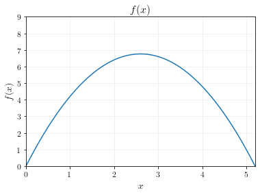
Suppose you’re given an arbitrary function, \(f(x)\). The function has the following graph:

What value of \(x\) maximizes \(f(x)\)? \(f(x)\) is maximized at the value of \(x\) where the slope of the function is flat.
Mathematical Insight
In single variable optimization, the maximum of a function is found at the point where the slope is exactly equal to zero.
It’s like climbing a mountain. To ascend, you follow the direction where the slope rises fastest. You know you’re at the peak when the point you’re standing on is flat and in every direction you look the land is sloping downwards away from you.
Slopes of functions
The slope of a function measures how fast the “output” changes as the “inputs” change.
In two dimensions, with \(y=f(x)\), the slope measures how fast \(y\) changes as \(x\) changes. You may have heard it explained as “rise over run”.
Most functions do not have a constant slope. The slope is different at each value of \(x\), just like how the slope of a mountain depends on your position on the mountain.
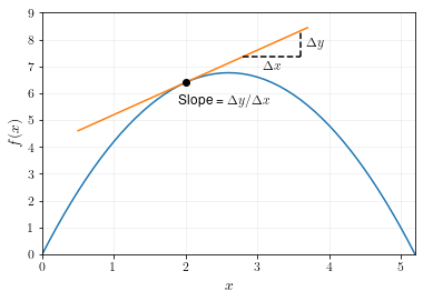
To calculate slope at a particular point, draw a straight line which just touches the function at that point, then calculate the slope of the line.
When a line is just touching a function at \(x\), we say that the line is tangent to the function at \(x\).
Example 1
The diagram below shows how to calculate the slope of the function at \(x=2\).
Example 2
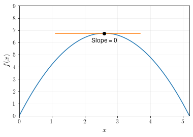
For the same function, we calculate slope at \(x=2.6\) (the maximum) and see that it’s zero.
Derivatives of functions
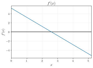
Since the slope of a function is different at every point, we can define another function that maps \(x\) to the slope of \(f(x)\). We call this function the derivative of \(f(x)\).
By convention, we notate the derivative of \(f(x)\) as \(f^\prime(x)\) or \(\frac{d}{dx} f(x)\). Both notations mean the same thing.
Example 3
The graphs below show the function \(f(x)\) and its derivative, \(f^\prime(x)\). The derivative shows the slope of \(f(x)\) at each value of \(x\). Notice how the slope is positive when \(x<2.6\), zero when \(x=2.6\), and negative when \(x>2.6\).
Derivative rules
To find the derivative of common functions, you can make use of the following rules.
| Main Function | Derivative of Function | |
| Constant Rule | \(f(x) = a\) | \(f^\prime(x) = 0\) |
| Constant Multiple Rule | \(f(x) = ag(x)\) | \(f^\prime(x) = ag^\prime(x)\) |
| Power Rule | \(f(x) = x^a\) | \(f^\prime(x) = ax^{a-1}\) |
| Log Rule | \(f(x) = \ln x\) | \(f^\prime(x) = 1/x\) |
| Sum Rule | \(f(x) = g(x) + h(x)\) | \(f^\prime(x) = g^\prime(x) + h^\prime(x)\) |
| Difference Rule | \(f(x) = g(x) - h(x)\) | \(f^\prime(x) = g^\prime(x) - h^\prime(x)\) |
| Chain Rule | \(f(x) = g[h(x)]\) | \(f^\prime(x) = g^\prime[h(x)] h^\prime(x)\) |
Example 4
Find the derivative of \(f(x) = 5.2x - x^2\). Then calculate the slope of \(f(x)\) when \(x=2\).
Answer.
\(f^\prime(x) = 5.2 - 2x\) (Apply the constant multiple rule, power rule, and difference rule.)
\(f^\prime(2) = 5.2 - 4 = 1.2\). So the slope of \(f(x)\) when \(x=2\) is 1.2.
Example 5
Find the derivative of \(f(x) = ax^2 + bx + c\). Then calculate the slope of \(f(x)\) when \(x=-1\)
Answer.
\[\begin{aligned} f^\prime(x) &= 2ax + b \\ f^\prime(-1) &= 2a(-1) + b = -2a + b \end{aligned}\]
Example 6
Find the derivative of \(f(x) = \ln( x^2 + 2x + 1)\).
Answer.
To do this, we need the chain rule. Write:
\[f(x) = g[h(x)]\]where:
\[\begin{aligned} g(x) &= \ln x \\ h(x) &= x^2 + 2x + 1 \\ \end{aligned}\]By the log rule:
\[g^\prime(x) = 1/x\]By the power rule and sum rule:
\[h^\prime(x) = 2x+2\]Finally, we use the chain rule:
\[\begin{aligned} f^\prime(x) &= g^\prime[ h(x) ] h^\prime(x) & \\ &= \frac{1}{x^2+2x+1} (2x+2) & \\ &= \frac{2x+2}{x^2+2x+1} \end{aligned}\]If you want, you could simplify this equation even further.
First order conditions
A function \(f(x)\) is maximized at the value of \(x\) for which the slope is flat. In other words, it is maximized at the value of \(x\) for which the derivative equals zero.
This gives us a strategy for finding the maximum of any single variable function. Find the \(x\) that solves the equation:
\[f^\prime(x) = 0\]This condition is known as the first order condition.
Example 7
In the above graphs, the equation of the function was:
\[f(x) = 5.2x - x^2\]At what value of \(x\) is \(f(x)\) maximized?
Answer.
First, we find the derivative:
\[f^\prime(x) = 5.2 - 2x\]Then, we find the \(x\) which solves:
\[f^\prime(x) = 0\]Solving the equation:
\[\begin{aligned} 5.2 - 2x &= 0 & \\ 5.2 &= 2x & \text{(Add 2x to both sides)} \\ 5.2/2 &= x & \text{(Divide both sides by 2)} \\ 2.6 &=x & \end{aligned}\]So \(f(x) = 5.2x - x^2\) is maximized at \(x=2.6\).
Example 8
A firm is deciding how much quantity \(q\) to produce. It can sell its output at a price of $10. The total cost of production is equal to \(q^2\).
Write a function that maps the firm’s choice of output, \(q\), into its profit. Then, find the choice of \(q\) which maximizes profit, and calculate the maximum possible profit.
Answer.
Profit function:
\[\Pi(q) = 10q - q^2\]Derivative of profit function:
\[\Pi^\prime(q) = 10 - 2q\]Solving the first order condition:
\[\begin{aligned} \Pi^\prime(q) &= 0 \\ 10 - 2q &=0 \\ 10 &= 2q \\ 5 &= q \end{aligned}\]So the profit is maximized when \(q=5\).
To calculate the profit, simply plug \(q=5\) back into \(\Pi(q)\).
\[\begin{aligned} \Pi(5) &= 10(5) - (5)^2 \\ &= 50 - 25 \\ &= 25 \end{aligned}\]So the maximum profit attainable is 25.
Example 9
Find the value of \(x\) that maximizes:
\[f(x) = a + bx - cx^2\]And find the value of \(f(x)\) at the maximum.
Answer.
First order condition:
\[\begin{aligned} b - 2cx &= 0 \\ b &= 2cx \\ \frac{b}{2c} &= x \end{aligned}\]Thus, \(f(x)\) is maximized at \(x = b/(2c)\).
To find the maximum value of \(f(x)\), plug the value of \(x=b/(2c)\) back into \(f(x)\):
\[f\left(\frac{b}{2c}\right) = a + b\left(\frac{b}{2c}\right) - c\left(\frac{b}{2c}\right)^2\]Which simplifies to:
\[f\left(\frac{b}{2c}\right) = a + \frac{b^2}{4c}\](Check the simplification yourself)


