Math Review
- Functions
- Graphing functions
- Supply and demand curves as functions
- Working with exponents
- Working with logs
Functions
A function is a mapping from one or more “input” variables to an “output” variable.
Example 1
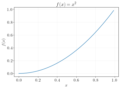
\[f(x) = x^2\]This maps \(x\) to the square of \(x\).
If \(x=2\), then \(f(x)=4\).
If \(x=3\), then \(f(x)=9\). And so on…
Example 2
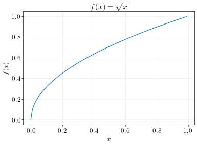
\[f(x) = \sqrt{x}\]This maps \(x\) to the square root of \(x\).
If \(x=4\), then \(f(x)=2\).
If \(x=9\), then \(f(x)=3\). And so on…
Example 3
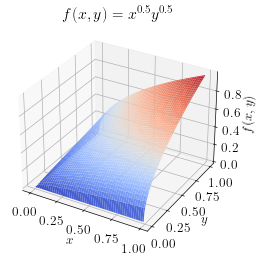
\[f(x,y) = x^{0.5}y^{0.5}\]If \(x=1\) and \(y=1\), then \(f(x,y)=1\).
If \(x=4\) and \(y=9\), then \(f(x,y)=6\). And so on…
Graphing functions
Functions can be visualized using graphs. A graph simply plots the different input values along with their output value.
Example 4
Example 5
Example 6
Supply and demand curves as functions
Supply curves and demand curves are functions.
The demand curve maps price onto quantity demanded. Let’s write \(q_d = f(p)\), where \(f\) is some arbitrary function.
The supply curve maps price onto quantity supplied. Let’s write \(q_s = g(p)\), where \(g\) is some arbitrary function.
The market is in equilibrium when \(q_d = q_s\). Thus, the price that equilibrates the market is the price that solves the equation: \(f(p) = g(p)\).
Example 7
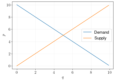
Supply and demand curves are defined by:
\[\begin{aligned} q_d &= 10 - p \\ q_s &= p \end{aligned}\]In equilibrium, \(q_d = q_s\), or \(10 - p = p\).
Solve:
\[\begin{aligned} 10-p&=p \\ 10&=2p & (\text{Add p to both sides})\\ 5&=p & (\text{Divide both sides by 2})\end{aligned}\]So the equilibrium price is 5 and the equilibrium quantity is 5.
The graph below illustrates.
Working with exponents
We’ll work a lot with exponents in this class. Exponents allow us to add curvature to functions that more realistically reflect economic forces like consumers’ utility functions and firms’ production functions.
To work with exponents, you need to memorize these rules:
| Zero Rule | \(x^0 = 1\) |
| Product Rule | \(x^a x^b = x^{a+b}\) |
| Quotient Rule | \(x^a / x^b = x^{a-b}\) |
| Power of a Product | \((xy)^a = x^a y^a\) |
| Power of a Fraction | \((x/y)^a = x^a / y^a\) |
| Power of a Power | \((x^a)^b = x^{ab}\) |
| Negative Exponent | \(x^{-a} = 1/x^a\) |
| Inverse Rule | \((x^a)^{1/a} = x\) |
Example 8
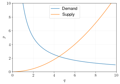
Supply and demand curves are defined by:
\[\begin{aligned} q_d &= 10/p \\ q_s &= 3p^{1/2} \end{aligned}\]Solve for the equilibrium price:
\[\begin{aligned} q_d &= q_s & \\ 10/p &= 3p^{1/2} & \\ 10 &= 3p^{1/2} p & \text{(Multiply p on both sides)} \\ 10/3 &= p^{1/2} p & \text{(Divide both sides by 3)} \\ 10/3 &= p^{3/2} & \text{(Apply product rule)} \\ (10/3)^{2/3} &= p & \text{(Apply inverse rule)} \end{aligned}\]Using a calculator, we calculate an equilibrium price of 2.23 and an equilibrium quantity of 4.48.
These supply and demand curves are plotted in the graph below.
Working with logs
It’s also quite common in economics to work with natural logs (the \(\ln\) function). The log function is useful because the difference in the log of two quantities is approximately equal to the percent change between the two quantities.
To work with logs, you’ll need to memorize these rules:
| Log of 1 | \(\ln 1 = 0\) |
| Product Rule | \(\ln (xy) = \ln x + \ln y\) |
| Quotient Rule | \(\ln (x/y) = \ln x - \ln y\) |
| Power Rule | \(\ln (x^a) = a \ln x\) |
| Inverse Rule 1 | \(e^{\ln x} = x\) |
| Inverse Rule 2 | \(\ln (e^x) = x\) |
| Difference Rule | \(\ln y - \ln x \approx (y-x)/x\) |
Here, \(e\) is Euler’s Number, a mathematical constant equal to 2.71828. Euler’s Number arises naturally out of the mathematics of compounding interest rates, and thus has many applications in economics and finance.
Example 9
Natural logs are useful for modeling supply and demand curves with constant elasticity. For example, suppose the demand curve is specified by:
\[\ln q_d = 10 - 2\ln p\]Using the difference rule, you can show that whenever price changes by \(+1\)%, then quantity demanded changes by \(-2\)%. This demand curve therefore has a constant elasticity of demand equal to \(-2\).
More generally, if:
\[\ln q_d = a - b\ln p\]Then the elasticity of demand is constant and equal to \(-b\).
