Economics Review
- The word marginal
- Principle of optimization
- Demand curves
- Supply curves
- Market equilibrium
- Consumer surplus
- Producer surplus
- Efficiency of competitive markets
- Deadweight loss
This lecture reviews the basic concepts from an introductory microeconomics course that you’ll need for this class.
The word marginal
We’ll be using the word marginal a lot. In economics, the “marginal X of Y” means “the additional amount of X that happens when Y is increased by an incremental amount”.
So, for example, the “marginal cost of production” means “the additional cost it takes to produce an additional unit of output”. And the “marginal benefit of consumption” means the “additional benefit gained from consuming an additional unit of goods”.
As we’ll see in the next two lectures, there’s a close association between the “marginal X of Y” and the “derivative of X with respect to Y”.
Principle of optimization
Suppose you are choosing how much of something, \(x\) to do. For example, how much of a good to consume if you’re a consumer, or how much to produce if you’re a producer.
There is a benefit and cost associated with every choice of \(x\). The principle of optimization says that you maximize your total benefit minus total cost when you choose \(x\) such that the marginal benefit of \(x\) equals the marginal cost of \(x\).
The reasoning is straightforward. If the marginal benefit of \(x\) exceeds the marginal cost, then the additional benefit you gain from an additional unit of \(x\) exceeds the cost. Which means you should do more of it. Which means your current choice is not optimal.
If the marginal benefit of \(x\) is lower than the marginal cost, then the additional cost of the incremental unit has already exceeded the benefit. You should have done less of it. Again, your current choice was not optimal.
Your current choice is only optimal if the marginal benefit exactly equals the marginal cost.
As we’ll see in the next two lectures, there’s a close association between this principle of optimization and what’s known in mathematical optimization as a “first order condition”.
Principle of Optimization
Total benefit minus total cost is maximized at the quantity where marginal benefit equals marginal cost.
Demand curves
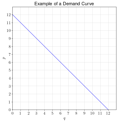
Definition. A demand curve shows the relationship between a commodity’s price and the quantity that will be demanded by consumers in a market.
Assumptions. In order for a demand curve to exist, it is assumed that the consumers in the market are price-takers, meaning that the behavior of a single consumer has no influence on the market price. This would be true, for example, if there are many consumers such that a single consumer constitutes only a tiny fraction of the total demand.
Relationship to marginal benefit. The demand curve not only shows the relationship between price and quantity demanded, it also shows the relationship between quantity consumed and the marginal benefit of consumption. This is because consumers will demand goods up to the quantity where the price equals the marginal benefit of consumption.
Supply curves
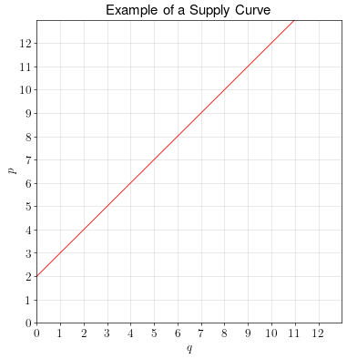
Definition. A supply curve shows the relationship between a commodity’s price and the quantity that will be produced and sold by producers (firms) in a market.
Assumptions. In order for a supply curve to exist, it is assumed that the producers in the market are price-takers, meaning that the behavior of a single producer has no influence on the market price. This would be true, for example, if there are many producers such that a single producer constitutes a tiny fraction of the total supply.
The assumption that producers are price-takers seems less realistic than the assumption that consumers are price-takers. Indeed, we’ll investigate models where producers are not price-takers later in the course.
Relationship to marginal cost. The supply curve not only shows the relationship between price and quantity supplied, it also shows the relationship between quantity produced and the marginal cost of production. This is because producers will produce goods up to the quantity where the price equals the marginal cost of production.
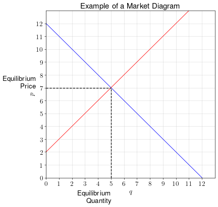
Market equilibrium
Price affects both the quantity demanded and the quantity supplied.
If price is too low, the quantity demanded will exceed the quantity supplied. Over time, the price of the good will be bid up.
If price is too high, the quantity supplied will exceed the quantity demanded. Over time, the price of the good will be bid down.
When the quantity supplied equals the quantity demanded, we say that the market is in equilibrium. It is at a point of stability in which we won’t predict further changes to the price unless the underlying supply and demand curves change.
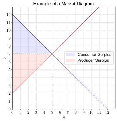
Consumer surplus
Consumer surplus is a measure of how much the consumers’ well-being is improved by participating in the market.
Because the demand curve is equal to the consumers’ marginal benefit curve, we can calculate consumer surplus by calculating the area under the demand curve and above the price. This area represents the total benefits derived from consumption minus the total price paid by the consumers.
Producer surplus
Producer surplus is a measure of how much the producers’ well-being is improved by participating in the market.
Because the supply curve is equal to the producers’ marginal cost curve, we can calculate producer surplus by calculating the area above the supply curve and below the price. This area represents the total revenue derived from sales minus the total cost paid by the firms.
Efficiency of competitive markets
In a competitive market with price-taking consumers and firms, the equilibrium of the market maximizes the total surplus (consumer surplus + producer surplus) available in the market.
This is because in the market equilibrium, price equals both marginal cost and marginal benefit. Thus, \(MB=MC\) in equilibrium, which means the total benefit minus the total cost in the market is maximized.
When total surplus is maximized, we say that the market is efficient.
Deadweight loss
Certain circumstances can result in the market becoming inefficient. For example, taxation, price controls, and monopoly power can all lead to the market inefficient.
If the market is inefficient, we call the loss in total surplus due to the inefficiency deadweight loss.
Example
Supply and demand in a market are defined by the following equations:
\[\begin{align} q_d &= 24 - \frac{4}{3}p \\ q_s &= 2p - 16 \end{align}\]
- Calculate the equilibrium price and quantity.
- Draw the supply and demand curve in the provided grid.
- Calculate the consumer and producer surplus.
Answer.
Calculate the equilibrium price and quantity.
Step 1. Write down the equilibrium condition and substitute in the equations.
\[\begin{align} q_d &= q_s \\ 24 - \frac{4}{3}p &= 2p - 16 \end{align}\]Step 2. Solve the equation for \(p\).
\[\begin{aligned} 24 - \frac{4}{3}p &= 2p - 16 & \\ 16 + 24 - \frac{4}{3}p &= 2p ~ ~ ~ ~ & \text{(Add 16 to both sides)} \\ 40 &= 2p + \frac{4}{3}p ~ ~ ~ ~ & \text{(Add 4/3 p to both sides)} \\ 40 &= \frac{10}{3}p ~ ~ ~ ~ & \text{(Simplify 2p + 4/3 p)} \\ p &= \frac{3}{10} \times 40 ~ ~ ~ ~ & \text{(Multiply both sides by 3/10}) \\ p &= 12 & \end{aligned}\]Step 3. Plug \(p=12\) into either the supply or the demand equation.
\[\begin{aligned} q_s &= 2p - 16 \\ &= 2\times 12 - 16 \\ &= 24 - 16 \\ &= 8 \end{aligned}\]Thus, in equilibrium, \(p=12\) and \(q=8\).
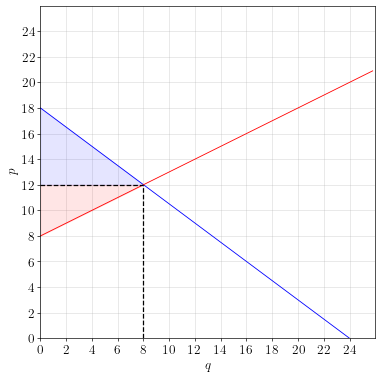
Draw the supply and demand curves in the provided grid.
To plot the curves, find the \(y\)-axis intercept for both demand curves, then draw a straight line to the equilibrium point.
Calculate the consumer and producer surplus.
As a reminder, the area of a triangle is:
\[\text{Area of a Triangle} = \frac{1}{2} \times \text{base} \times \text{height}\]The consumer surplus is the area of the blue triangle and producer surplus is the area of the red triangle.
\[\begin{aligned} CS &= \frac{1}{2} \times 8 \times 6 = 24 \\ PS &= \frac{1}{2} \times 8 \times 4 = 16 \end{aligned}\]